MiniCPM Series
MiniCPM
Model Wind Tunnel Experiments (MWTE)
MWTE contains three parts
- Hyper-parameters
- Optimal Batch-size Scaling
- Optimal Learning Rate Stability
Warmup-Stable-Decay (WSD) Learning Rate Scheduler
Especially, the WSD LRS contains three stages:
the warmup stage (whose end step is denoted by W),
the stable training stage (whose end step is denoted by T),
and the remaining decay stage.
\[ W S D(T ; s)=\left\{\begin{array}{l} \frac{s}{W} \eta, \quad s<W \\ \eta, \quad W<s<T \\ f(s-T) \eta, \quad T<s<S \end{array}\right. \]
\[ \text { where } 0<f(s-T) \leq 1 \text { is a decreasing function about } s \]
??? \[ f(s-S)= 0.5^{(s-S)/T} \] 其中T为退火的半衰期,我们设置为T=8000步。
Metrics:
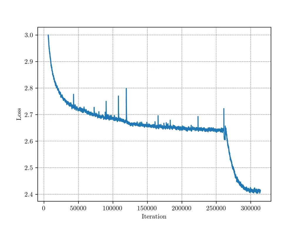
- Loss Decreases Dramatically in Decay Stage
- 10% Steps are Enough - in the subsequent training experiments, we use a decay of about 10% to ensure full convergence. \(WSD(D,0.1D)\).
- Effective Data Scaling with WSD LRS - Previously, if the average cost of training one model size on one data size is C, then conducting the scaling experiments with m model sizes and m data sizes takes approximately O(m2 )C. In this section, we introduce the utilization of the WSD scheduler as an effective approach to explore the scaling law with linear cost (O(mC)). 说白了就是stable 阶段没变化,可以一直续更长的总步数
Two Stage Pre-training Strategy
- 稳定训练阶段(warmup+stable):batchsize为3.93M,Max Learning Rate为0.01。粗粒度数据集
- 退火阶段(Decay):学习率降低到1e-3,采用指数退火𝑓(𝑠−𝑆)=𝜂×0.5^(𝑠−𝑆)/𝑇,其中T为退火的半衰期,设置为8000步。在退火阶段加入SFT阶段的高质量数据
Training Stages
- Stable Training Stage. 和上文一样。We utilize around 1T data (see Section 11 for data distribution), with the majority of the data sourced from open datasets. We use the optimal configuration discovered during the model wind tunnel experiments, WSD LRS, with a batch size of 3.93 million and a max learning rate of 0.01.
- Decay Stage. 预训练中的退火阶段。
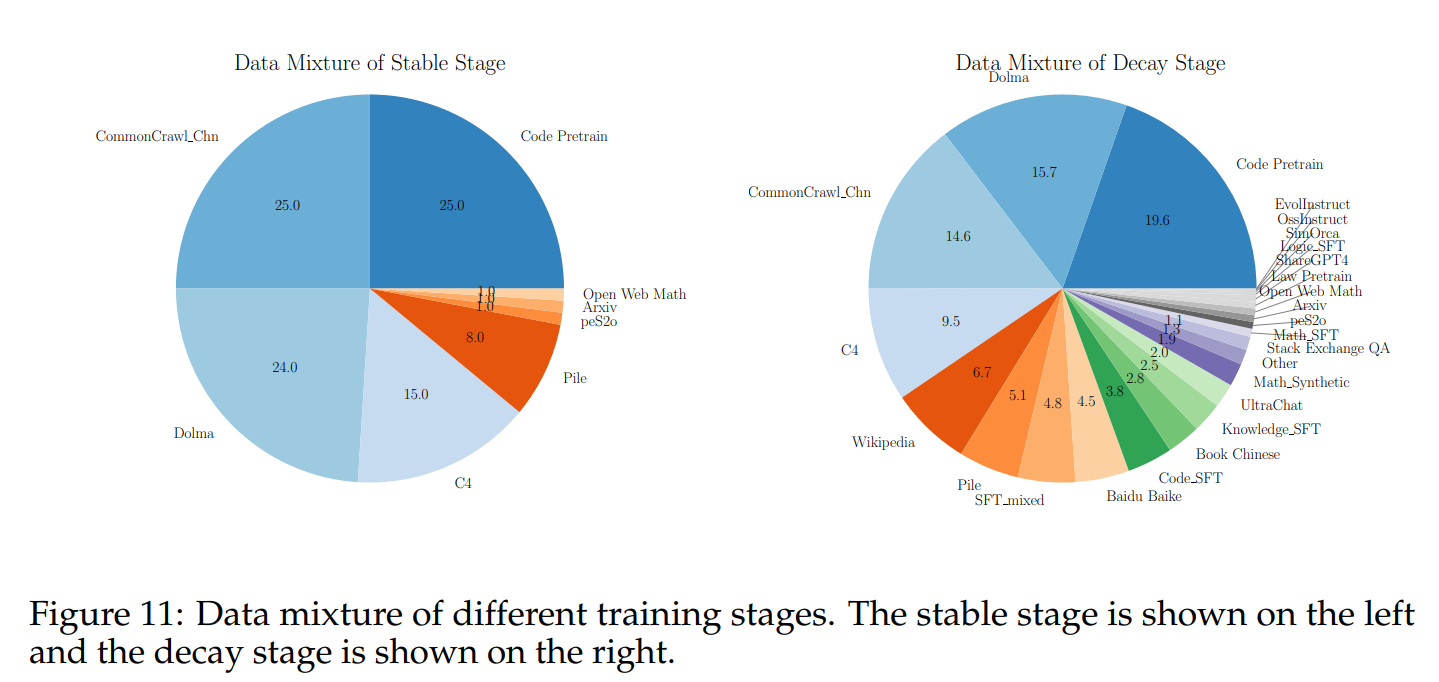
SFT Stage. We find it still necessary to conduct a separate SFT phase. We utilize SFT data similar to the annealing phase excluding pre-training data and train with approximately 6 billion tokens. The learning rate for SFT is aligned with the one at the end of annealing, and a WSD Scheduler with exponential decay is also employed.
alignment
- SFT的学习率衔接上退火结束的学习率,为1e-3,同样使用了WSD Scheduler。
- 在SFT之后,我们采用DPO对模型进行进一步的人类偏好对齐。在这一阶段,我们采用UltraFeedback作为主要的对齐数据集,并内部构建了一个用于增强模型代码和数学能力的偏好数据集。我们进行了一个Epoch的DPO训练,学习率为1e-5且使用Cosine Scheduler。更多DPO和数据设置细节可以可见我们 UltraFeedback 论文。
测试
整体评测使用了面壁智能的开源工具UltraEval,其数据集选取了常用的权威数据集,包括:
- 英文,选取了MMLU
- 中文,选取了CMMLU、C-Eval
- 代码,选取了HumanEval、MBPP
- 数学,选取了GSM8K、MATH
- 问答,选取了HellaSwag、ARC-E、ARC-C
- 逻辑,选取了BBH
量化:MiniCPM-sft/dpo-int4
为进一步降低MiniCPM的计算开销,使用GPT-Q方法将MiniCPM量化为int4版本。相较于bfloat16版本与float32版本,使用int4版本时,模型存储开销更少,推理速度更快。量化模型时,我们量化Embedding层、LayerNorm层外的模型参数。 \[ \text { scale }=\frac{\max (\mathbf{w})-\min (\mathbf{w})}{2^4-1}, \text { zero }=-\frac{\min (\mathbf{w})}{\text { scale }}-2^3 \] 采用int4量化时,数值范围为 \([-2^3,2^3-1]\),数值范围为\(2^4-1\)。zero为缩放后的偏移量,因为原参数期望可能并不为零。因此当\(\frac{min}{scale}\)不为\(-2^3\)时,就手动水平调整它的值让它缩放到下界。
依照上述放缩系数和零点,\(\bold{w}\)量化后为 \[ \bold{\hat w} = quant(\bold{w}) = round(\frac{\bold{w}}{scale} +zero) \] 其中取整函数\(round()\)为向最近整数取整。反量化时,操作方式如下: \[ dequant(\bold{\hat w}) = scale \cdot (\bold{\hat w} - zero) \] 使用GPT-Q方法进行量化时,在标注数据\(\bold{X}\)上最小化量化误差\(||\bold{WX} - dequant(\bold{\hat W}\bold{X})||^2_2\), 并循环对矩阵的未量化权重进行如下更新,其中\(q\)是当前量化的参数位置,\(\bold{F}\)为未量化权重,\(\bold{H}_\bold{F}\)是量化误差的Hessian矩阵。
多模态:MiniCPM-V
基于MiniCPM,我们构建了一个支持中英双语对话的端侧多模态模型MiniCPM-V。该模型可以接受图像和文本输入,并输出文本内容。MiniCPM-V 的视觉模型部分由 SigLIP-400M 进行初始化,语言模型部分由 MiniCPM 进行初始化,两者通过perceiver resampler进行连接。
MiniCPM-V有三个突出特点:
- 高效推理:MiniCPM-V 可以高效部署在大多数 GPU 显卡和个人电脑,甚至手机等边缘设备上。在图像编码表示方面,我们基于perciever resampler将每个图像压缩表示为64个token,显著少于其他基于MLP架构的多模态模型的token数量(通常大于 512)。这使得MiniCPM-V 可以在推理过程中以更低的存储成本和更高的运算速度进行推理。
- 性能强劲:在多个基准测试(包括 MMMU、MME 和 MMbech 等)中,MiniCPM-V 在同规模模型中实现了最佳性能,超越了基于 Phi-2 构建的现有多模态大模型。MiniCPM-V 在部分数据集上达到了与 9.6B Qwen-VL-Chat 相当甚至更好的性能。
- 双语支持:MiniCPM-V是首个支持中英文双语能力的可边缘部署的多模态端侧大模型。该能力是通过跨语言泛化多模态能力高效实现的,这项技术来自我们的 ICLR 2024 splotlight论文。
MiniCPM-V 模型的训练分为 2 个基本阶段:
- 预训练阶段: 我们使用 300M 中英图文对数据进行视觉和语言基本概念的对齐,并学习大规模多模态世界知识。
- 指令微调阶段: 我们一共使用了6M 多任务问答数据、1M 纯文本数据、1M 多模态对话数据进行指令微调,进一步对齐并激发多模态基础能力。
详细训练与微调过程也可见我们 ICLR 2024 splotlight论文。
MiniCPM-V
The model comprises three key modules: the visual encoder, compression layer, and LLM.
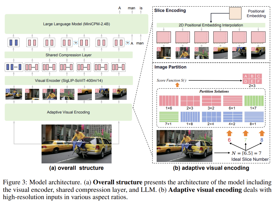
Adaptive Visual Encoding
To this end, we take advantage of the adaptive visual encoding method proposed by LLaVA-UHD [107].
Image partition
we first calculate the ideal number of slices based on the input image size.
Given an image with resolution \(\left(W_I, H_I\right)\) and a ViT pre-trained on images with resolution \(\left(W_v, H_v\right)\), we calculate the ideal slice number \(N=\left\lceil\frac{W_T \times H_I}{W_v \times H_v}\right\rceil\). Then, we choose the combination of rows \(n\) and columns \(m\) from the set \(\mathbb{C}_N=\{(m, n) \mid m \times n=N, m \in \mathbb{N}, n \in \mathbb{N}\}\). A good partition \((m, n)\) should result in slices that match well with ViT's pre-training setting. To achieve this, we use a score function to evaluate each potential partition: \[ S(m, n)=-\left|\log \frac{W_I / m}{H_I / n}-\log \frac{W_v}{H_v}\right| \]
We select the partition with the highest score from all possible candidates: \[ m^*, n^*=\underset{(m, n) \in \overline{\mathbb{C}}}{\arg \max } S(m, n), \] where \(\overline{\mathbb{C}}\) is the possible \((m, n)\) combinations with the product \(N\). However, when \(N\) is a prime number, the feasible solutions can be limited to \((N, 1)\) and \((1, N)\). Therefore, we additionally introduce \(\mathbb{C}_{N-1}\) and \(\mathbb{C}_{N+1}\), and set \(\overline{\mathbb{C}}=\mathbb{C}_{N-1} \cup \mathbb{C}_N \cup \mathbb{C}_{N+1}\). In practice, we set \(N<10\), supporting 1.8 million pixels (e.g., \(1344 \times 1344\) resolution) at most during encoding. Although we can encompass more image slices for higher resolutions, we purposely impose this resolution upper-bound, since it already well covers most real-world application scenarios, and the benefit of further increasing encoding resolution is marginal considering the performance and overhead.
Slice encoding
\(W_I / m\) or \(H_I / n\) is not exactly the same as \(W_v\) or \(H_v\), resize. Subsequently, we interpolate the ViT’s position embeddings to adapt to the slice’s ratio.
We also include the original image as an additional slice to provide holistic information about the entire image.
Token Compression
After visual encoding, each slice is encoded into 1,024 tokens, where 10 slices can yield over 10k tokens collectively. To manage this high token count, we employ a compression module comprising of one-layer cross-attention and a moderate number of queries, with 2D positions informed [7]. In practice, the visual tokens of each slice are compressed into 64 queries for MiniCPM V1&2 and 96 tokens for MiniCPM-Llama3-V 2.5 through this layer.
Spatial Schema
To indicate each slice’s position relative to the whole image, inspired by [9], we additionally introduce a spatial schema. We first wrap tokens of each slice by two special tokens \(\text{<slice>}\) and \(\text{<\slice>}\), and then employ a special token \(\text{\n}\) to separate slices from different rows.
Pre-training
In this phase, we utilize large-scale image-text pairs for MLLM pre-training. The primary goal of this phase is to align the visual modules (i.e., visual encoder and compression layer) with the input space of the LLM and learn foundational multimodal knowledge.
The pre-training phase is further divided into 3 stages.
warm up the compression layer.
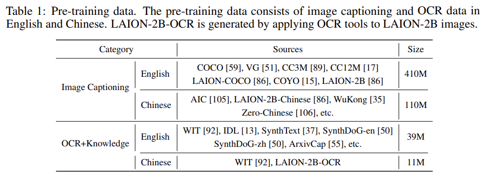
We randomly initialize the compression layer and train this module in stage-1, keeping other parameters frozen. The visual encoder’s resolution is set to 224×224, which is the same as the visual encoder’s pre-training setting. To warm up the compression layer, we randomly select 200M data from the Image Captioning data in Table 1. Data cleaning is performed to remove image-text pairs with poor correlation and ill-formatted text data, ensuring the data quality.
extend the input resolution of the pre-trained visual encoder.
In stage-2, we extend the image resolution from 224×224 to 448×448. The whole visual encoder is trained, leaving other parameters frozen. To extend the pre-trained resolution, we additionally select 200M data from the Image Captioning data in Table 1.
train the visual modules using the adaptive visual encoding strategy.
During the stage-3 training, both the compression layer and the visual encoder are trained to adapt to the language model embedding space. The LLM is kept frozen.
Different from the previous stages with only image captioning data, during the highresolution pre-training stage, we additionally introduce OCR data to enhance the visual encoders’ OCR capability.
Caption Rewriting. Image-text pairs sourced from the Web [86, 15] can suffer from quality issues in the caption data, including non-fluent content, grammatical errors, and duplicated words. Such low-quality data can lead to unstable training dynamics. To address the issue, we introduce an auxiliary model for low-quality caption rewriting. The rewriting model takes the raw caption as input and is asked to convert it into a question-answer pair. The answer from this process is adopted as the updated caption. In practice, we leverage GPT-4 [14] to annotate a small number of seed samples, which are then used to fine-tune an LLM for the rewriting task.
Data Packing. Samples from different data sources usually have different lengths. The high variance of sample lengths across batches will lead to inefficiency in memory usage and the risk of out-of-memory (OOM) errors. To address the issue, we pack multiple samples into a single sequence with a fixed length. By truncating the last sample in the sequence, we ensure uniformity in sequence lengths, facilitating more consistent memory consumption and computational efficiency. Meanwhile, we modify the position ids and attention masks to avoid interference between different samples. In our experiments, the data packing strategy can bring 2~3 times acceleration in the pre-training phase.
Multilingual Generalization. Multimodal capability across multiple languages is essential for serving users from broader communities. Traditional solutions involve extensive multimodal data collection and cleaning, and training for the target languages. Fortunately, recent findings from VisCPM [41] have shown that the multimodal capabilities can be efficiently generalized across languages via a strong multilingual LLM pivot. This solution largely alleviates the heavy reliance on multimodal data in low-resource languages. In practice, we only pre-train our model on English and Chinese multimodal data, and then perform a lightweight but high-quality multilingual supervised fine-tuning to align to the target languages. Despite its simplicity, we find the resultant MiniCPMLlama3-V 2.5 can achieve good performance in over 30 languages as compared with significantly larger MLLMs.
Supervised Fine-tuning
SFT phase mainly utilizes high-quality datasets annotated by either human lablers or strong models such as GPT-4.
We categorize the SFT data into two parts. Part-1 focuses on bolstering the models’ basic recognition capabilities, while part-2 is tailored to enhance their capabilities in generating detailed responses and following human instructions.
part-1 data consists of the traditional QA/captioning datasets with relatively short response lengths, which helps enhance the model’s basic recognition capabilities.
part-2 encompasses datasets featuring long responses with complex interactions, either in text or multimodal context.
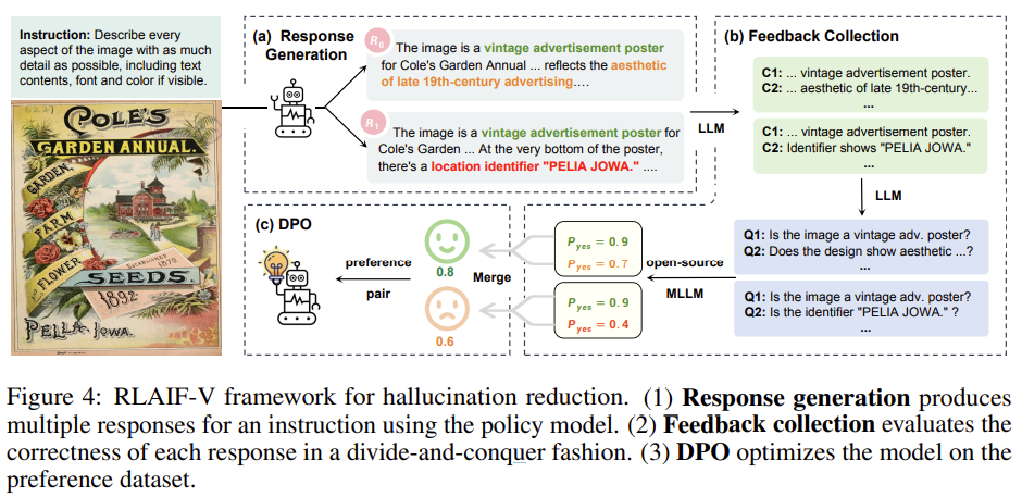
RLAIF-V
we employ the recent RLAIF-V [112] approach (Fig. 4), where the key is to obtain scalable high-quality feedback from open-source models for direct preference optimization (DPO) [82].