Stable Diffusion
High-Resolution Image Synthesis with Latent Diffusion Models
Key points:
- Training Diffusion Models in latent space, which allows for the first time to reach a near-optimal point between complexity reduction and detail preservation.
- Introducing cross-attention layers into the model architecture, which turn diffusion models into powerful and flexible generators for general conditioning inputs such as text or bounding boxes and high-resolution synthesis becomes possible in a convolutional manner.
Method:
Perceptual Image Compression
More precisely, given an image \(x \in \mathbb{R}^{H \times W \times 3}\) in RGB space, the encoder \(\mathcal{E}\) encodes \(x\) into a latent representation \(z=\mathcal{E}(x)\), and the decoder \(\mathcal{D}\) reconstructs the image from the latent, giving \(\tilde{x}=\mathcal{D}(z)=\mathcal{D}(\mathcal{E}(x))\), where \(z \in \mathbb{R}^{h \times w \times c}\). Importantly, the encoder downsamples the image by a factor \(f=H / h=W / w\), and we investigate different downsampling factors \(f=2^m\), with \(m \in \mathbb{N}\).
Latent Diffusion Models
Generative Modeling of Latent Representations With our trained perceptual compression models consisting of \(\mathcal{E}\) and \(\mathcal{D}\), we now have access to an efficient, low-dimensional latent space in which high-frequency, imperceptible details are abstracted away.
Conditioning Mechanisms
Image Text cross attention. Q: Image, K,V: Text. So the projection layer K have to shape the text to image space.
To pre-process \(y\) from various modalities (such as language prompts) we introduce a domain specific encoder \(\tau_\theta\) that projects \(y\) to an intermediate representation \(\tau_\theta(y) \in \mathbb{R}^{M \times d_\tau}\), which is then mapped to the intermediate layers of the UNet via a cross-attention layer implementing \(\operatorname{Attention}(Q, K, V)=\operatorname{softmax}\left(\frac{Q K^T}{\sqrt{d}}\right) \cdot V\), with \[ Q=W_Q^{(i)} \cdot \varphi_i\left(z_t\right), K=W_K^{(i)} \cdot \tau_\theta(y), V=W_V^{(i)} \cdot \tau_\theta(y) \] Here, \(\varphi_i\left(z_t\right) \in \mathbb{R}^{N \times d_\epsilon^i}\) denotes a (flattened) intermediate representation of the UNet implementing \(\epsilon_\theta\)
and \(W_V^{(i)} \in\) \(\mathbb{R}^{d \times d_\epsilon^i}, W_Q^{(i)} \in \mathbb{R}^{d \times d_\tau} \& W_K^{(i)} \in \mathbb{R}^{d \times d_\tau}\) are learnable projection matrices [35, 94].
See Fig. 3 for a visual depiction.
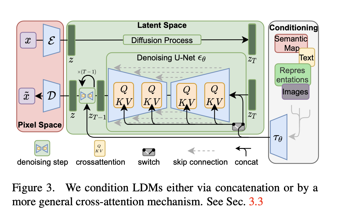
Based on image-conditioning pairs, we then learn the conditional LDM via \[ L_{L D M}:=\mathbb{E}_{\mathcal{E}(x), y, \epsilon \sim \mathcal{N}(0,1), t}\left[\left\|\epsilon-\epsilon_\theta\left(z_t, t, \tau_\theta(y)\right)\right\|_2^2\right] \] where both \(\tau_\theta\) and \(\epsilon_\theta\) are jointly optimized via Eq. 3. This conditioning mechanism is flexible as \(\tau_\theta\) can be parameterized with domain-specific experts, e.g. (unmasked) transformers [94] when \(y\) are text prompts (see Sec. 4.3.1)