DDIM
Denoising diffusion implicit models (DDIMs)
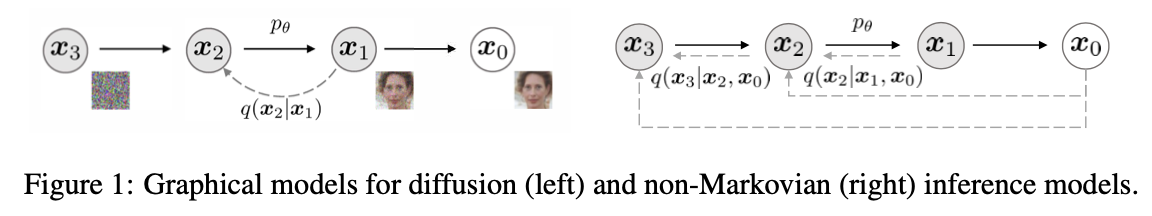
We generalize DDPMs via a class of non-Markovian diffusion processes that lead to the same training objective. These non-Markovian processes can correspond to generative processes that are deterministic, giving rise to implicit models that produce high quality samples much faster.
First, DDIMs have superior sample generation quality compared to DDPMs, when we accelerate sampling by 10× to 100× using our proposed method. Second, DDIM samples have the following “consistency” prop- erty, which does not hold for DDPMs: if we start with the same initial latent variable and generate several samples with Markov chains of various lengths, these samples would have similar high-level features. Third, because of “consistency” in DDIMs, we can perform semantically meaningful image interpolation by manipulating the initial latent variable in DDIMs, unlike DDPMs which interpolates near the image space due to the stochastic generative process.
Recal in DDPM, the loss only depands on the marginals \(q(\mathbf{x}_t \mid \mathbf{x}_0)\) , but not directly on the joint \(q\left(\boldsymbol{x}_{1: T} \mid \boldsymbol{x}_0\right)\). \[ \mathbb{E}_q[\underbrace{D_{\mathrm{KL}}\left(q\left(\mathbf{x}_T \mid \mathbf{x}_0\right) \| p\left(\mathbf{x}_T\right)\right)}_{L_T}+\sum_{t>1} \underbrace{D_{\mathrm{KL}}\left(q\left(\mathbf{x}_{t-1} \mid \mathbf{x}_t \mathbf{x}_0\right) \| p_\theta\left(\mathbf{x}_{t-1} \mid \mathbf{x}_t\right)\right)}_{L_{1: T-1}} \underbrace{-\log p_\theta\left(\mathbf{x}_0 \mid \mathbf{x}_1\right)}_{L_0}] \] Since there are many inference distributions (joints) with the same marginals, we explore alternative inference processes that are non-Markovian, which leads to new generative processes.
To summarize what DDIM aims to achieve:
- DDIM aims to construct a sampling distribution \(p(x_{t-1} \mid x_t, x_0)\) that does not rely on the first-order Markov assumption.
- DDIM aims to maintain the forward inference distribution \(q(x_t \mid x_0) = \mathcal{N}(x_t; \sqrt{\bar{\alpha}_t} x_0, (1-\bar{\alpha}_t) \mathbf{I})\).
Non-Markovian Forward Process
The method involves constructing a sampling distribution such that its inference distribution matches that of DDPM, enabling the formulation of an equation.
- Constructing the sampling distribution. This sampling distribution has three free variables: \(\lambda\), \(k\), and \(\sigma_t\).
\[ p\left(x_{t-1} \mid x_t, x_0\right) = \mathcal{N}\left(x_{t-1} ; \lambda x_0 + k x_t, \sigma_t^2 \mathbf{I}\right) \]
- Target inference distribution:
\[ q\left(x_t \mid x_0\right) = \mathcal{N}\left(x_t ; \sqrt{\bar{\alpha}_t} x_0, (1-\bar{\alpha}_t) \mathbf{I}\right) \]
- Using mathematical induction, we only need to ensure that \(t - 1\) remains valid for \(q(x_{t-1}|x_0)\), i.e., solving:
\[ \int_{x_t} p\left(x_{t-1} \mid x_t, x_0\right) q\left(x_t \mid x_0\right) dx_t = q\left(x_{t-1} \mid x_0\right) \]
We can solve this using the method of undetermined coefficients: \[ x_{t-1}=\lambda x_0+k x_t+\sigma \epsilon_{t-1}^{\prime} \]
\[ x_t=\sqrt{\bar{\alpha}_t} x_0+\sqrt{\left(1-\bar{\alpha}_t\right)} \epsilon_t^{\prime} \]
Therefore \[ \begin{aligned} x_{t-1} & =\lambda x_0+k\left(\sqrt{\bar{\alpha}_t} x_0+\sqrt{\left(1-\bar{\alpha}_t\right)} \boldsymbol{\epsilon}_t^{\prime}\right)+\sigma_t \boldsymbol{\epsilon}_{t-1}^{\prime} \\ & =\left(\lambda+k \sqrt{\bar{\alpha}_t}\right) x_0+\underbrace{k \sqrt{\left(1-\bar{\alpha}_t\right)} \boldsymbol{\epsilon}_t^{\prime}+\sigma_t \boldsymbol{\epsilon}_{t-1}^{\prime}}_{\text { additivity of normal distributions }} \\ x_{t-1} &= \left(\lambda+k \sqrt{\bar{\alpha}_t}\right) x_0 + \sqrt{\left(k^2\left(1-\bar{\alpha}_t\right)+\sigma_t^2\right)} \bar{\epsilon}_{t-1} \end{aligned} \] Since \(q\left(x_{t-1} \mid x_0\right)=\mathcal{N}\left(x_{t-1} ; \sqrt{\bar{\alpha}_{t-1}} x_0,\left(1-\bar{\alpha}_{t-1}\right) \mathbf{I}\right)\), we can derive that \[ x_{t-1}=\sqrt{\bar{\alpha}_{t-1}} x_0+\sqrt{\left(1-\bar{\alpha}_{t-1}\right)} \boldsymbol{\epsilon}_{t-1} \] By equating the corresponding terms, we can obtain two equations for the three unknowns.Clearly, there are infinitely many sets of solutions that can satisfy these equations. In DDIM, \(\sigma_t\) is considered a variable: \[ \left\{\begin{array}{l} \lambda+k \sqrt{\bar{\alpha}_t}=\sqrt{\bar{\alpha}_{t-1}} \\ k^2\left(1-\bar{\alpha}_t\right)+\sigma_t^2=1-\bar{\alpha}_{t-1} \end{array} \Rightarrow\left(\begin{array}{l} \lambda^* \\ k^* \\ \sigma_t^* \end{array}\right)=\left(\begin{array}{c} \sqrt{\bar{\alpha}_{t-1}}-\sqrt{\bar{\alpha}_t} \sqrt{\frac{1-\bar{\alpha}_{t-1}-\sigma_t^2}{1-\bar{\alpha}_t}} \\ \sqrt{\frac{1-\bar{\alpha}_{t-1}-\sigma_t^2}{1-\bar{\alpha}_t}} \\ \sigma_t \end{array}\right)\right. \] Since the forward process remains unchanged, we can directly use the noise prediction model trained by DDPM. The sampling process is as follows: \[ x_{t-1}=\sqrt{\bar{\alpha}_{t-1}} x_0+\sqrt{1-\bar{\alpha}_{t-1}-\sigma_t^2} \epsilon_t +\sigma_t z \] we can replace \(\epsilon_t\) with \(x_0\): \[ x_{t-1}=\sqrt{\bar{\alpha}_{t-1}} x_0+\sqrt{1-\bar{\alpha}_{t-1}-\sigma_t^2} \frac{x_t-\sqrt{\bar{\alpha}_t} x_0}{\sqrt{1-\bar{\alpha}_t}}+\sigma_t z \]
There are two special cases worth noting:
- When \(\sigma_t=\sqrt{\frac{1-\bar{\alpha}_{t-1}}{1-\bar{\alpha}_t}} \times \sqrt{1-\frac{\bar{\alpha}_t}{\bar{\alpha}_{t-1}}}\), the generation process is consistent with DDPM.
- When \(\sigma_t=0\), the noise added during the sampling process is 0. Given \(z=x_t \sim \mathcal{N}(0, \mathbf{I})\), the sampling process becomes deterministic. The generative model in this case is an implicit probabilistic model. The authors refer to the diffusion model under this condition as the denoising diffusion implicit model (DDIM). The sampling recursion formula in this case is:
\[ x_{t-1}=\sqrt{\bar{\alpha}_{t-1}} \underbrace{\frac{x_t-\sqrt{1-\bar{\alpha}_t} \epsilon_\theta\left(x_t, t\right)}{\sqrt{\bar{\alpha}_t}}}_{\text {Predicted } x_0}+\underbrace{\sqrt{1-\bar{\alpha}_{t-1}} \epsilon_\theta\left(x_t, t\right)}_{\text {Direction of } x_0} \]
Accelerated generation process
\(\tau\) is an increasing sub-sequence of \([1, \ldots, T]\) of length \(S\). Therefore, \(\tau_i\) is a number within \(T\).
The forward process is not on all the latent variables \(x_{1:T}\), but on a subset \(\{x_{\tau_i}\}\), \(i \in {1, \cdots, S}\), \(1 \leq \tau_i \leq T\) \[ q\left(\mathbf{x}_{\tau_i} \mid \mathbf{x}_0\right)=\mathcal{N}\left(\mathbf{x}_{\tau_i} ; \sqrt{\bar{\alpha}_{\tau_i}} \mathbf{x}_0,\left(1-\bar{\alpha}_{\tau_i}\right) \mathbf{I}\right) \]
The generative process now samples latent variables according to reversed ( \(\tau\) ), which we term (sampling) trajectory. Because we user no markovian assumption. \[ x_{\tau_{s-1}}=\sqrt{\bar{\alpha}_{\tau_{s-1}}} \frac{x_{\tau_s}-\sqrt{1-\bar{\alpha}_{\tau_s}} \epsilon_\theta\left(x_{\tau_s}, t_{\tau_s}\right)}{\sqrt{\bar{\alpha}_{\tau_s}}}+\sqrt{1-\bar{\alpha}_{\tau_{s-1}}} \epsilon_\theta\left(x_{\tau_s}, t_{\tau_s}\right) \]