iDDPM
improved loss
variance \[ \Sigma_\theta\left(x_t, t\right)=\exp \left(v \log \beta_t+(1-v) \log \tilde{\beta}_t\right) \] First component learns mean, second learns variance \[ L_{\text {hybrid }}=L_{\text {simple }}+\lambda L_{\mathrm{vlb}} \]
- Predict \(v\): the output of model channel \(C\) doubles. First part of \(C\) predict mean, and the second part of \(C\) predict \(v\)
- Predict variance: the second part of \(C\) predict log variance (since model will output negative values)
1 | if self.model_var_type == ModelVarType.LEARNED: # Predict log variance |
mean
the Equation 12 of original paper is wrong. what is did in the code is \[ \begin{align} x_t &= \sqrt{\overline{\alpha}_t} x_0+\sqrt{1-\overline{\alpha}_t} \varepsilon_t \\ x_0 &= \frac{1}{\sqrt{\overline{\alpha}_t}} (x_t - \sqrt{1-\overline{\alpha}_t} \epsilon_t) \\ x_0 &= \frac{1}{\sqrt{\overline{\alpha}_t}} x_t - \epsilon_t \sqrt{\frac{1}{\overline{\alpha}_t} - 1} \end{align} \]
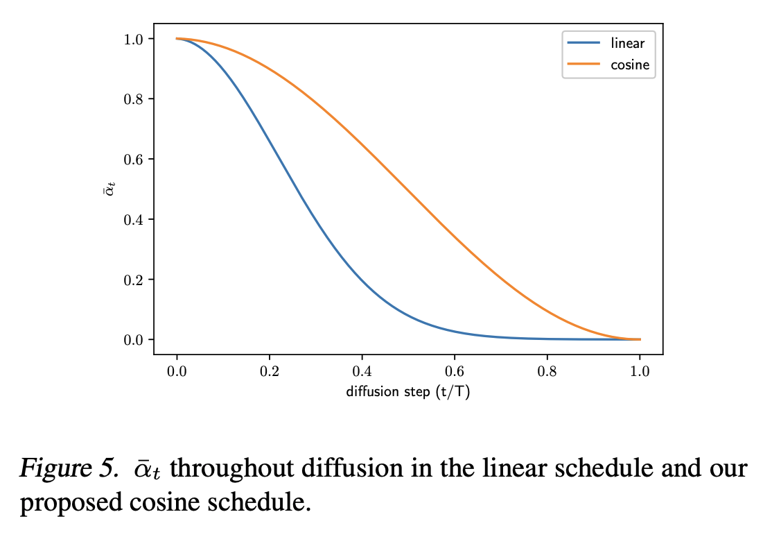
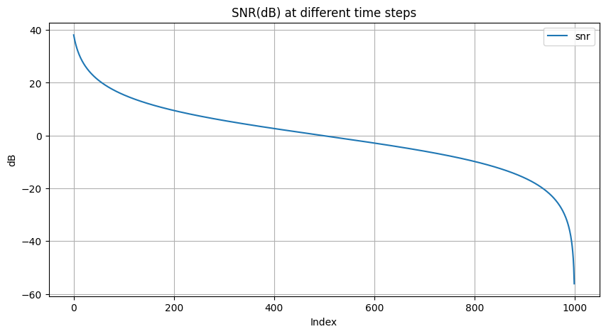
improved noise schedule
Use linear schedule will lead to noisier images earlier on the forward process
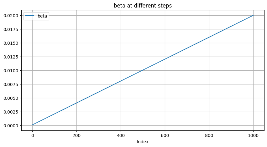
- Linear: starts from \(\beta_t\)
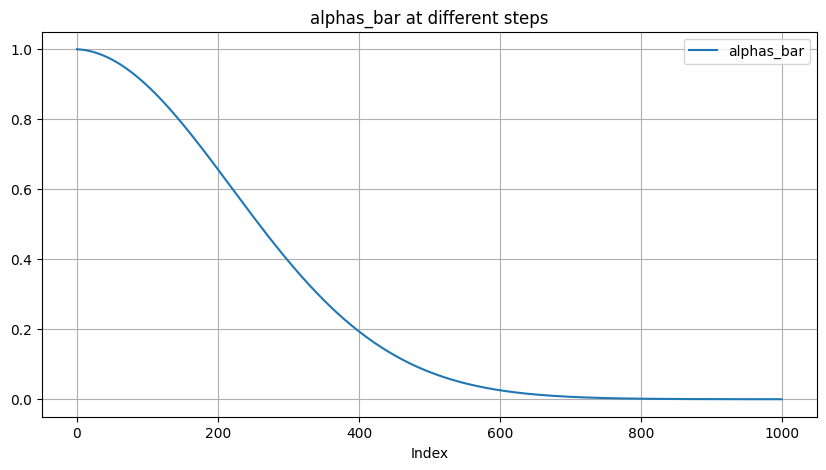
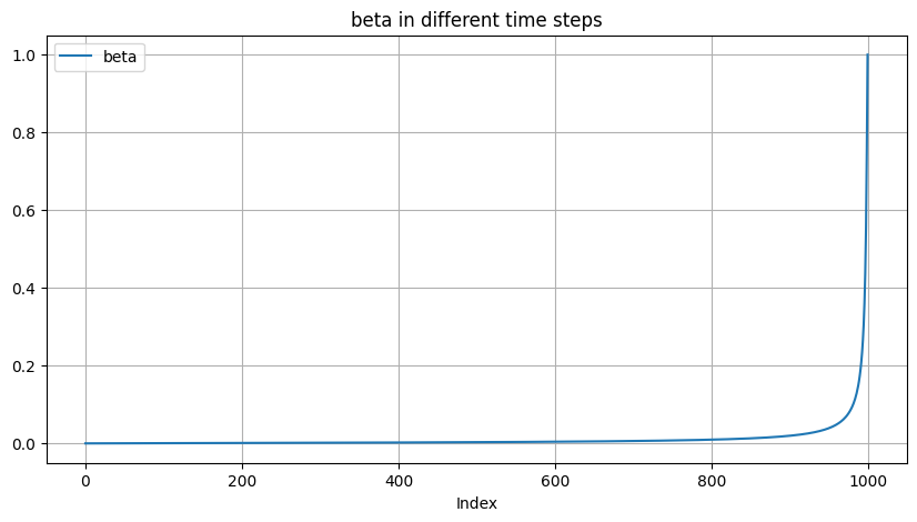
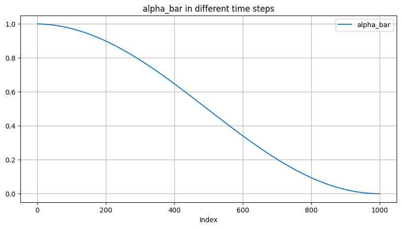
- Cosine: starts from \(\bar{\alpha}_t\)
To go from this definition to variances \(\beta_t\), we note that \(\beta_t=1-\frac{\bar{\alpha}_t}{\bar{\alpha}_{t-1}}\). In practice, we clip \(\beta_t\) to be no larger than 0.999 to prevent singularities at the end of the diffusion process near \(t=T\).
We use a small offset \(s\) to prevent \(\beta_t\) from being too small near \(t=0\), since we found that having tiny amounts of noise at the beginning of the process made it hard for the network to predict \(\epsilon\) accurately enough. In particular, we selected \(s\) such that \(\sqrt{\beta_0}\) was slightly smaller than the pixel bin size \(1 / 127.5\), which gives \(s=0.008\). We chose to use \(\cos ^2\) in particular because it is a common mathematical function with the shape we were looking for. This choice was arbitrary, and we expect that many other functions with similar shapes would work as well. \[ \bar{\alpha}_t=\frac{f(t)}{f(0)}, \quad f(t)=\cos \left(\frac{t / T+s}{1+s} \cdot \frac{\pi}{2}\right)^2 \]
linear
.png)
cosine
improved Unet
For unet model, see this post: