Development of Unet in Diffusion Models

Vannila Unet

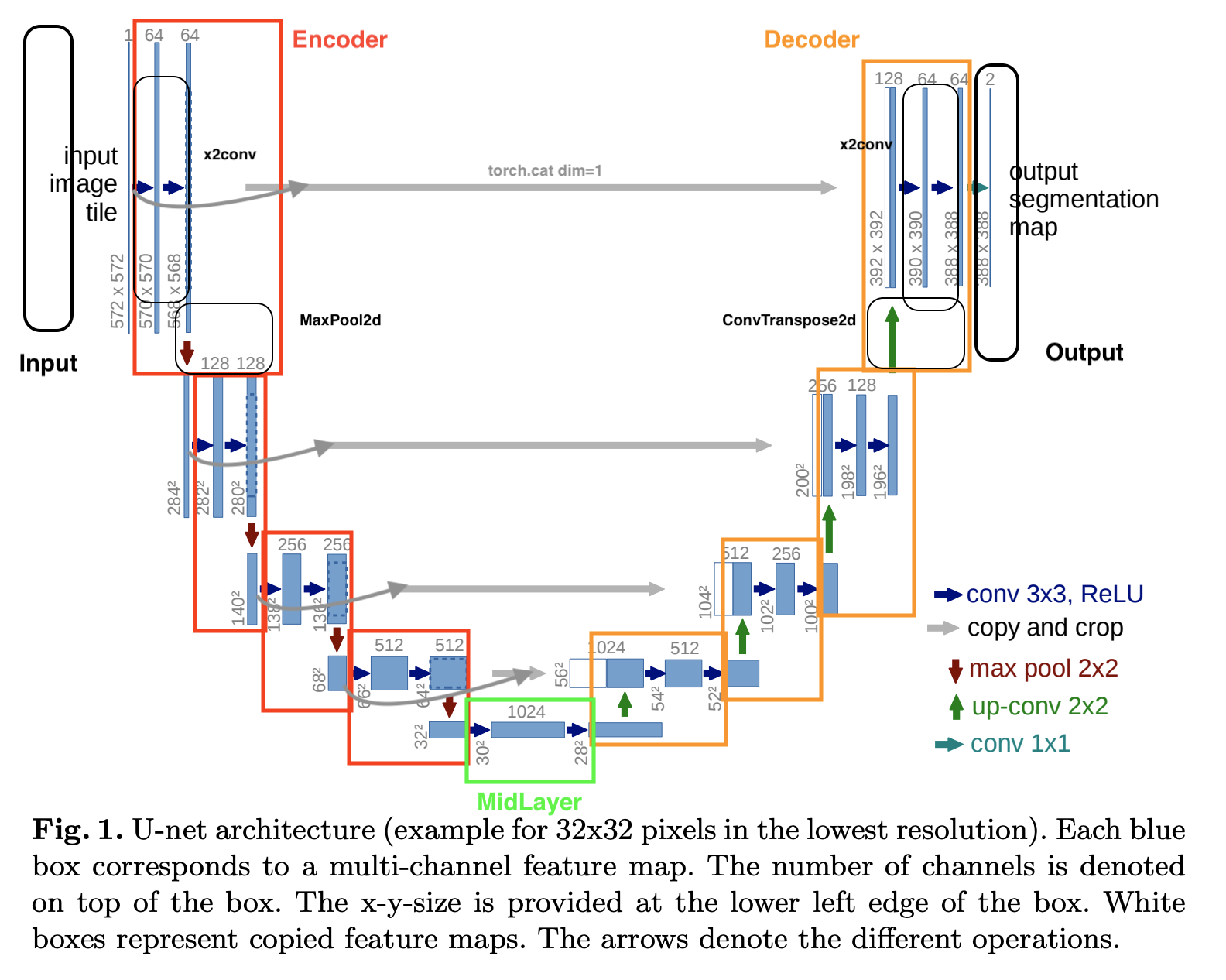
Notes

1. nn.ReLU(inplace=True) the ReLU activation function modifies the input data directly instead of creating a new copy of the data to store the results. So it can only be used in sequential structer since after relu, the original x has already been changed.

This code is not exactly the same as the original paper, but it a more modern style.

from base import BaseModel
import torch
import torch.nn as nn
import torch.nn.functional as F
from itertools import chain
from base import BaseModel
from utils.helpers import initialize_weights, set_trainable
from itertools import chain
from models import resnet


def x2conv(in_channels, out_channels, inner_channels=None):
    inner_channels = out_channels // 2 if inner_channels is None else inner_channels
    down_conv = nn.Sequential(
        nn.Conv2d(in_channels, inner_channels, kernel_size=3, padding=1, bias=False),
        nn.BatchNorm2d(inner_channels),
        nn.ReLU(inplace=True),
        nn.Conv2d(inner_channels, out_channels, kernel_size=3, padding=1, bias=False),
        nn.BatchNorm2d(out_channels),
        nn.ReLU(inplace=True))
    return down_conv

class encoder(nn.Module):
    def __init__(self, in_channels, out_channels):
        super(encoder, self).__init__()
        self.down_conv = x2conv(in_channels, out_channels)
        self.pool = nn.MaxPool2d(kernel_size=2, ceil_mode=True)

    def forward(self, x):
        x = self.down_conv(x)
        x = self.pool(x)
        return x

class decoder(nn.Module):
    def __init__(self, in_channels, out_channels):
        super(decoder, self).__init__()
        self.up = nn.ConvTranspose2d(in_channels, in_channels // 2, kernel_size=2, stride=2)
        self.up_conv = x2conv(in_channels, out_channels)

    def forward(self, x_copy, x, interpolate=True):
        x = self.up(x)

        if (x.size(2) != x_copy.size(2)) or (x.size(3) != x_copy.size(3)):
            if interpolate:
                # Iterpolating instead of padding
                x = F.interpolate(x, size=(x_copy.size(2), x_copy.size(3)),
                                mode="bilinear", align_corners=True)
            else:
                # Padding in case the incomping volumes are of different sizes
                diffY = x_copy.size()[2] - x.size()[2]
                diffX = x_copy.size()[3] - x.size()[3]
                x = F.pad(x, (diffX // 2, diffX - diffX // 2,
                                diffY // 2, diffY - diffY // 2))

        # Concatenate
        x = torch.cat([x_copy, x], dim=1)
        x = self.up_conv(x)
        return x

class UNet(BaseModel):
    def __init__(self, num_classes, in_channels=3, freeze_bn=False, **_):
        super(UNet, self).__init__()

        self.start_conv = x2conv(in_channels, 64)
        self.down1 = encoder(64, 128)
        self.down2 = encoder(128, 256)
        self.down3 = encoder(256, 512)
        self.down4 = encoder(512, 1024)

        self.middle_conv = x2conv(1024, 1024)

        self.up1 = decoder(1024, 512)
        self.up2 = decoder(512, 256)
        self.up3 = decoder(256, 128)
        self.up4 = decoder(128, 64)
        self.final_conv = nn.Conv2d(64, num_classes, kernel_size=1)
        self._initialize_weights()

        if freeze_bn:
            self.freeze_bn()

    def _initialize_weights(self):
        for module in self.modules():
            if isinstance(module, nn.Conv2d) or isinstance(module, nn.Linear):
                nn.init.kaiming_normal_(module.weight)
                if module.bias is not None:
                    module.bias.data.zero_()
            elif isinstance(module, nn.BatchNorm2d):
                module.weight.data.fill_(1)
                module.bias.data.zero_()

    def forward(self, x):
        x1 = self.start_conv(x)
        x2 = self.down1(x1)
        x3 = self.down2(x2)
        x4 = self.down3(x3)
        x = self.middle_conv(self.down4(x4))

        x = self.up1(x4, x)
        x = self.up2(x3, x)
        x = self.up3(x2, x)
        x = self.up4(x1, x)

        x = self.final_conv(x)
        return x

    def get_backbone_params(self):
        # There is no backbone for unet, all the parameters are trained from scratch
        return []

    def get_decoder_params(self):
        return self.parameters()

    def freeze_bn(self):
        for module in self.modules():
            if isinstance(module, nn.BatchNorm2d): module.eval()

iDDPM (DDPM)

Code

Zero Convolution

Q: If the weight of a conv layer is zero, the gradient will also be zero, and the network will not learn anything. Why "zero convolution" works? A: This is wrong. Let us consider a very simple \[ y=w x+b \] and we have \[ \partial y / \partial w=x, \partial y / \partial x=w, \partial y / \partial b=1 \] and if \(w=0\) and \(x \neq 0\), then \[ \partial y / \partial w \neq 0, \partial y / \partial x=0, \partial y / \partial b \neq 0 \] which means as long as \(x \neq 0\), one gradient descent iteration will make \(w\) non-zero. Then \[ \partial y / \partial x \neq 0 \] so that the zero convolutions will progressively become a common conv layer with non-zero weights.

At the end of self.embedding_layers and self.out_layers , there will a zero convolution, for example:

self.out_layers = nn.Sequential(
  normalization(self.out_channels),
  SiLU(),
  nn.Dropout(p=dropout),
  zero_module(
    conv_nd(dims, self.out_channels, self.out_channels, 3, padding=1)
  ),
)

def zero_module(module):
    """
    Zero out the parameters of a module and return it.
    """
    for p in module.parameters():
        p.detach().zero_()
    return module

since the output of self.embed add a none zero output with self.in_layers , the gradient will backprop with no trouble.

Scale before QKV

The comment, “More stable with f16 than dividing afterwards,” implies that multiplying the scaling factors to Q and K before computing their dot products provides more numerical stability than performing the dot product first and then dividing by a value (like the square root of the feature dimension). This is particularly true when using half-precision floating points (i.e., float16 or f16). Scaling helps prevent numerical overflow or underflow during computations. Using einsum for such operations effectively combines multiple steps into one, reducing cumulative errors and improving efficiency and precision.

class QKVAttention(nn.Module):
    """
    A module which performs QKV attention.
    """

    def forward(self, qkv):
        """
        Apply QKV attention.

        :param qkv: an [N x (C * 3) x T] tensor of Qs, Ks, and Vs.
        :return: an [N x C x T] tensor after attention.
        """
        ch = qkv.shape[1] // 3
        q, k, v = th.split(qkv, ch, dim=1)
        scale = 1 / math.sqrt(math.sqrt(ch))
        weight = th.einsum(
            "bct,bcs->bts", q * scale, k * scale
        )  # More stable with f16 than dividing afterwards
        weight = th.softmax(weight.float(), dim=-1).type(weight.dtype)
        return th.einsum("bts,bcs->bct", weight, v)

torch.einsum, originating from the Einstein Summation Convention, is a method that provides a succinct way of expressing multiple summations (like tensor dot products, matrix multiplication, transposing, etc.) on tensors.

The code snippet weight = th.einsum("bct,bcs->bts", q * scale, k * scale) uses the torch.einsum function, which is a powerful tool for specifying how to operate on multiple tensors. torch.einsum, originating from the Einstein Summation Convention, is a method that provides a succinct way of expressing multiple summations (like tensor dot products, matrix multiplication, transposing, etc.) on tensors.

Detailed Explanation

In the code weight = th.einsum("bct,bcs->bts", q * scale, k * scale):

• Input tensors: q * scale and k * scale are the scaled query (Q) and key (K) tensors.
• einsum expression: "bct,bcs->bts" can be interpreted as:
  • bct represents the first tensor (Q) with three dimensions: b for batch size, c for channels, and t for sequence length.
  • bcs represents the second tensor (K) with three dimensions: b for batch size, c for channels, and s for sequence length (which can differ from t, representing a different sequence length).
  • -> bts indicates the dimensions of the output tensor: b for batch size, t from Q’s sequence length, and s from K’s sequence length.
• Operation: This expression denotes that for each batch b, every time step t of Q is dot-producted with every time step s of K, resulting in a tensor that sums these dot products.

Time step embedding

Vanilla Transformers

The vanilla positional encoding in transformers is: \[ \begin{aligned} P E_{(p o s, 2 i)} & =\sin \left(p o s / 10000^{2 i / d_{\text {model }}}\right) \\ P E_{(p o s, 2 i+1)} & =\cos \left(p o s / 10000^{2 i / d_{\text {model }}}\right)\end{aligned} \]

\[ freq = \frac{1}{10000^{\frac{2i}{d}}}=10000^{-\frac{2i}{d}}=e^{-\frac{2i}{d}log{10000}} \]

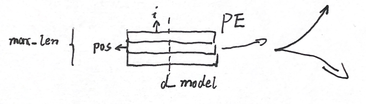
where \(PE\) is a matrix, like below. \(POS\) is the position of on token, and \(i\) is the index of values in one position embedding. We can see that the value inside the sine or cosine increases from up to down and decreases from left to right. Therefore:

• Denominator: \([1, 10000]\)
• numerator: \([0, max\_seq\_len]\)

Since \(\frac{\pi}{2} \approx \frac{3.14}{2} = 1.57\), so at most time, the input of \(PE\) is monotonically increasing from up to down and monotonically decrease from left to right.

#pytorch
import torch
import math
max_len = 3
d_model = 4
pe = torch.zeros(3, 4)
position = torch.arange(0, max_len).unsqueeze(1)
div_term = torch.exp(torch.arange(0, d_model, 2) *
                             -(math.log(10000.0) / d_model))
pe[:, 0::2] = torch.sin(position * div_term)
pe[:, 1::2] = torch.cos(position * div_term)
pe

iDDPM's time step embedding

The only different part is that it puts cosine after sine, not separate consine and sine one by one line any more. \[ freq = \frac{1}{10000^{\frac{2i}{d}}}=10000^{-\frac{2i}{d}}=e^{-\frac{2i}{d}log{10000}} \]

\[ args=pos*freq \]

\[ \begin{aligned} P E_{(p o s, i)} & = \sin \left(p o s / 10000^{i / dim}\right), \cos \left(p o s / 10000^{i / dim} \right)\end{aligned} \, i \in [0, dim//2] \]

\[ \begin{aligned} P E_{(p o s, i)} & = \sin \left(p o s / 10000^{i / dim}\right), \cos \left(p o s / 10000^{i / dim} \right)\end{aligned} ,0 \; if \, i\%2 \,\; \;i \in [0, dim//2] \]

def timestep_embedding(timesteps, dim, max_period=10000):
    """
    Create sinusoidal timestep embeddings.

    :param timesteps: a 1-D Tensor of N indices, one per batch element.
                      These may be fractional.
    :param dim: the dimension of the output.
    :param max_period: controls the minimum frequency of the embeddings.
    :return: an [N x dim] Tensor of positional embeddings.
    """
    half = dim // 2
    freqs = th.exp(
        -math.log(max_period) * th.arange(start=0, end=half, dtype=th.float32) / half  # from 1 to 1/T, 
    ).to(device=timesteps.device)
    args = timesteps[:, None].float() * freqs[None]
    embedding = th.cat([th.cos(args), th.sin(args)], dim=-1)
    if dim % 2:
        embedding = th.cat([embedding, th.zeros_like(embedding[:, :1])], dim=-1)
    return embedding

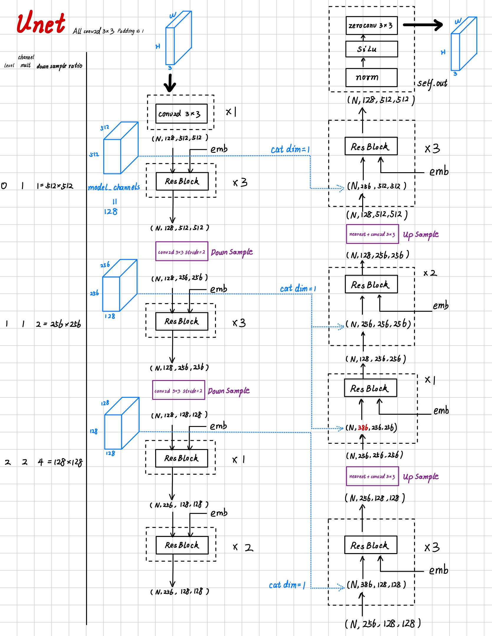
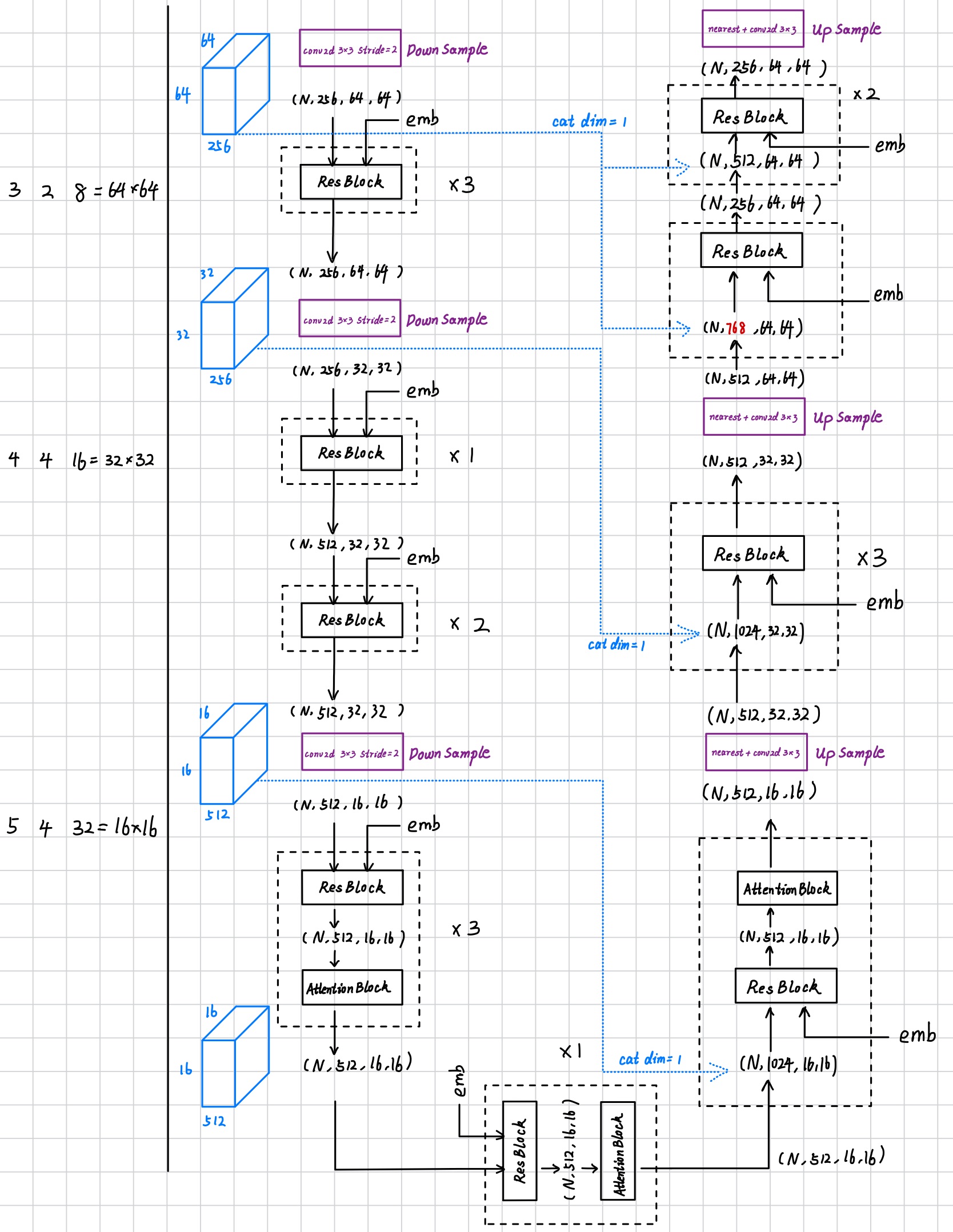
Network Figures

I hand wirte the figure about the work flow of Unet and some important blocks.

Overview & Time Embed

This time embed block is used to preprocess the time embedding rather than generating raw time embedding.

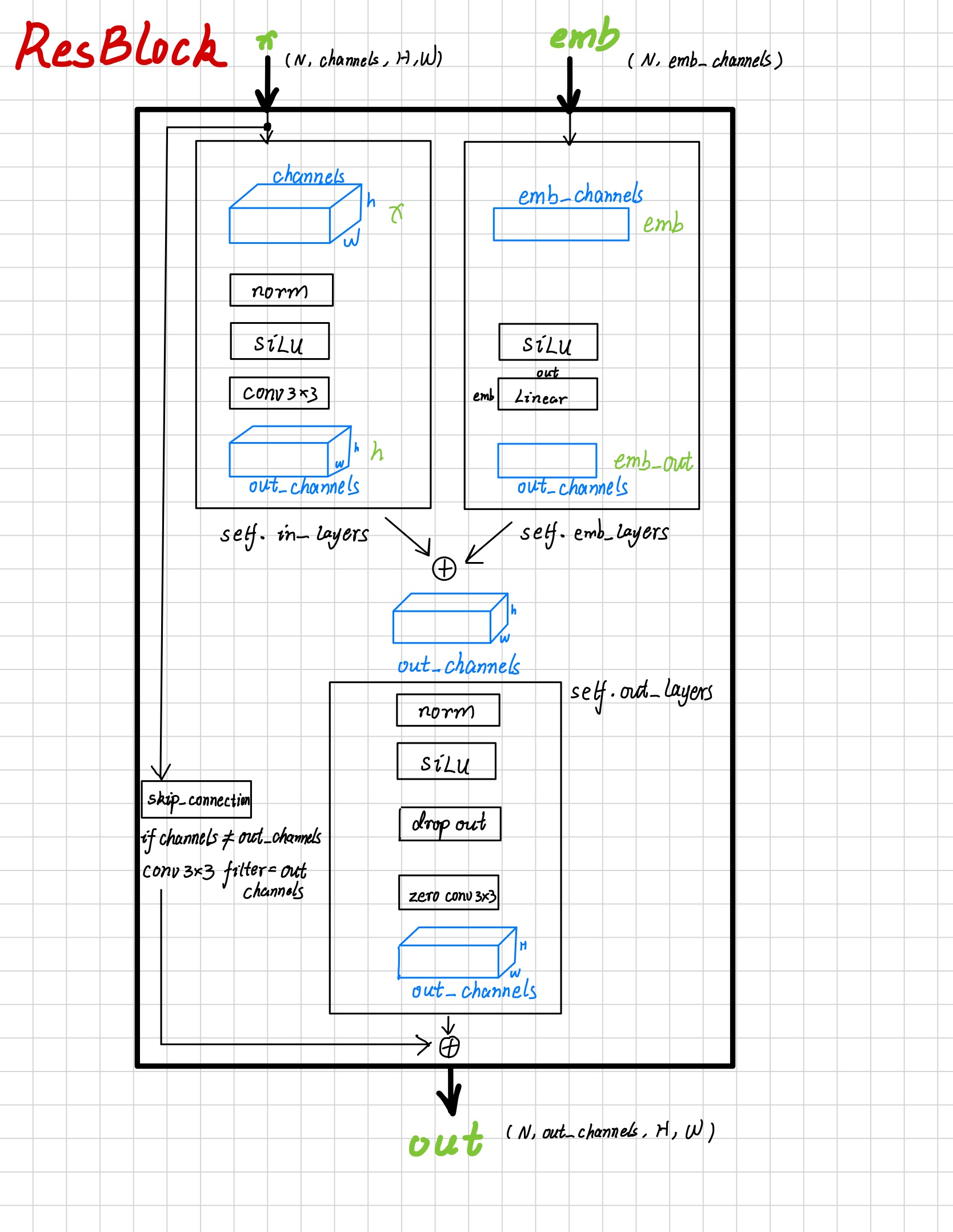
ResBlock

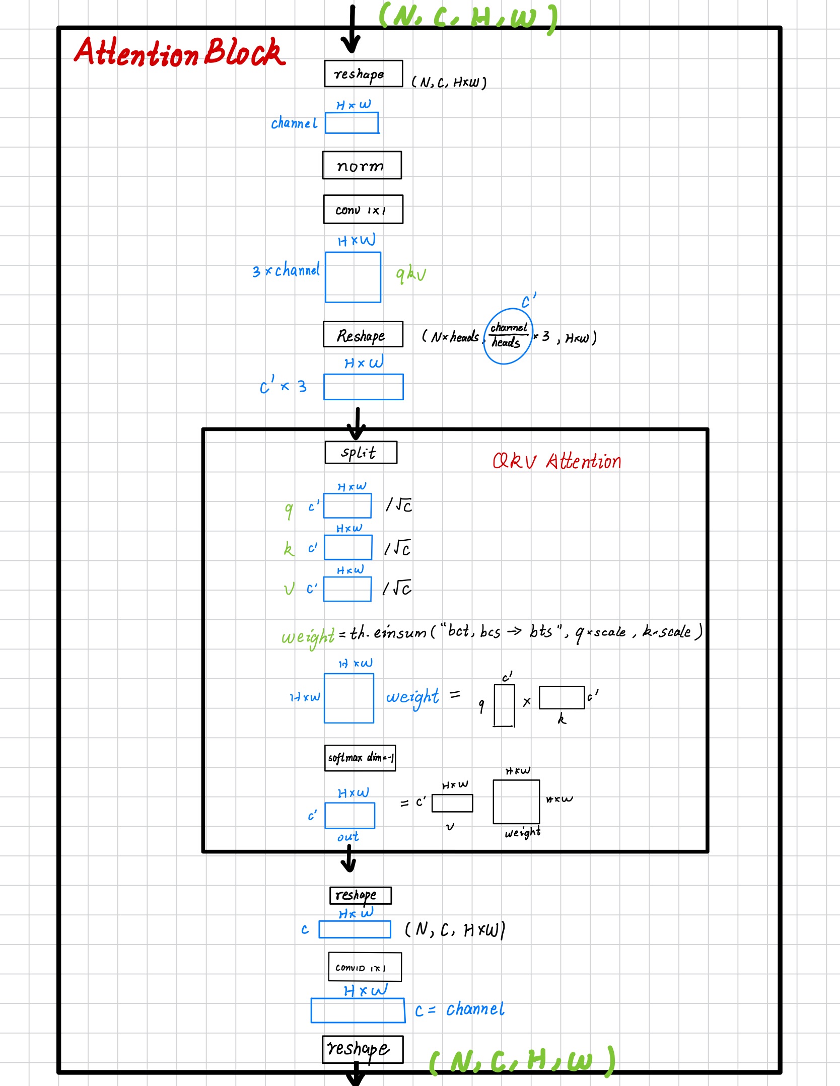
Attention Block

Unet