Neural Ordinary Differential Equations
Neural Ordinary Differential Equations
preliminary
ODE
An Ordinary Differential Equation (ODE) is an equation that involves one independent variable and its derivatives, describing the rate of change of one or more unknown functions. A general form of an n-th order ODE is: \[ F\left(t, y, y^{\prime}, y^{\prime \prime}, \ldots, y^{(n)}\right)=0 \] where: - \(t\) is the independent variable (often representing time). - \(y=y(t)\) is the unknown function. - \(y^{\prime}, y^{\prime \prime}, \ldots, y^{(n)}\) are the derivatives of \(y\) with respect to \(t\). - \(F\) is a given function involving \(t, y\), and its derivatives.
If the equation can be written explicitly as below, then it is called an explicit ODE.
\[ y^{(n)}=f\left(t, y, y^{\prime}, \ldots, y^{(n-1)}\right) \]
However, not every ODE can be converted to an explicit ODE. Some ODEs are inherently implicit, meaning that the highest-order derivative cannot be easily or explicitly solved in terms of the lower-order terms
Example:
\[ \left(y^{\prime \prime}\right)^2+y^{\prime}+t=0 \]
If we try to isolate \(y^{\prime \prime}\) :
\[ y^{\prime \prime}=\sqrt{-y^{\prime}-t} \]
Since taking a square root introduces ambiguity (positive and negative roots), this equation does not have a unique explicit form.
Classification of ODEs
Based on Order
- First-order ODE: Involves only the first derivative \(y'\)
- Second-order ODE: Involves the second derivative \(y''\)
- Higher-order ODE: Involves third or higher derivatives
Based on Linearity
Linear ODE: Can be written as: \[ a_n(t) y^{(n)}+a_{n-1}(t) y^{(n-1)}+\cdots+a_1(t) y^{\prime}+a_0(t) y=g(t) \] where \(a_i(t)\) are functions of \(t\), and \(g(t)\) is the nonhomogeneous term.
Nonlinear ODE: If \(y\) or its derivatives appear with nonlinear terms (e.g., squared, multiplied together, trigonometric functions), the equation is nonlinear.
\[ y^{\prime}+y^2=t \]
IVP for ODEs
An Initial Value Problem (IVP) for an Ordinary Differential Equation (ODE) is a problem where the solution to the differential equation is required to satisfy specific initial conditions.
An IVP consists of: 1. A differential equation of the form:
\[ y^{(n)}=f\left(t, y, y^{\prime}, \ldots, y^{(n-1)}\right) \]
- A set of initial conditions at \(t=t_0\):
\[ y\left(t_0\right)=y_0, \quad y^{\prime}\left(t_0\right)=y_1, \quad \ldots, \quad y^{(n-1)}\left(t_0\right)=y_{n-1} \]
The goal is to find a function \(y(t)\) that satisfies both the differential equation and the given initial conditions.
IVP Example for First-Order ODE \[ y' = f(t, y) = t \]
\[ y = \frac{1}{2}t^2 + C \]
given \(y(t_0)\) and \(t_0\), we can derive that: \[ y = \frac{1}{2}t^2 + y(t_0) - \frac{1}{2}t_0^2 \]
Numerical Methods
For many IVPs, finding an analytical solution is difficult or impossible, so we use numerical methods, such as:
Runge-Kutta Methods (RK4)
Adaptive Step-Size Methods (RK45)
Euler's Method \[ y_{n+1}=y_n+h f\left(t_n, y_n\right) \]
Euler’s Method
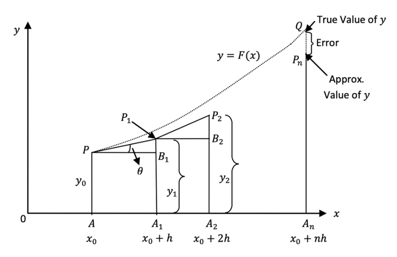
Euler's method is a simple numerical technique used to approximate the solution of first order initial value problems (IVPs) for ordinary differential equations (ODEs). It is a first-order method, meaning its error decreases linearly with smaller step size.
Euler’s method is based on the idea of using the tangent line at a known point to approximate the next point in the solution.
Given a first-order ODE: \[ \frac{d y}{d t}=f(t, y), \quad y\left(t_0\right)=y_0 \]
Euler's method estimates the solution at discrete points by using the recurrence formula:
\[ y_{n+1}=y_n+h f\left(t_n, y_n\right) \]
where: - \(y_n\) is the approximate solution at \(t_n\) - \(h\) is the step size, - \(f\left(t_n, y_n\right)\) is the derivative (slope), - \(t_{n+1}=t_n+h\).
This formula is derived from the Taylor series expansion but only keeps the first-order term.
Step-by-Step Explanation of Euler's Method
Choose the initial condition: Given \(y\left(t_0\right)=y_0\), set \(t_0\) and \(y_0\).
Choose a step size \(h\) : Smaller \(h\) gives more accuracy but requires more computations.
Iterate using Euler's formula:
Compute \(y_1, y_2, y_3, \ldots\) until reaching the desired \(t_{\text {final }}\).
Plot or store the results for analysis.
Abstract
Introduction
Models such as residual networks, recurrent neural network decoders, and normalizing flows build complicated transformations by composing a sequence of transformations to a hidden state:
<img src="https://minio.yixingfu.net/blog/2025-03-25/de6d5a512f10b8a4be505514181e41caf984c13f19045e854ed571977db7a1f2.png" width="30%">\[ \mathbf{y}_{t+1}=\mathbf{y}_t+f\left(\mathbf{y}_t, \theta_t\right),\quad \Delta t=1 \]
where \(t \in\{0 \ldots T\}\) and \(\mathbf{h}_t \in \mathbb{R}^D\). These iterative updates can be seen as an Euler discretization of a continuous transformation (Lu et al., 2017; Haber and Ruthotto, 2017; Ruthotto and Haber, 2018).
What happens as we add more layers and take smaller
steps? In the limit, we parameterize the continuous dynamics of
hidden units using an ordinary differential equation (ODE) specified by
a neural network:
\[
\frac{\mathbf{y}(t+\Delta t) - \mathbf{y}(t)}{\Delta t} =
f(\mathbf{y}(t), \theta, t)
\]
\[ \frac{d\mathbf{y}(t)}{dt} = \lim_{\Delta t \rightarrow 0} \frac{\mathbf{y}(t+\Delta t) - \mathbf{y}(t)}{\Delta t} =f(\mathbf{y}(t), \theta, t) \]
Which is exactly the form of first order ODE: \[ \mathbf{y}' = f(\mathbf{y}, \theta, t) \]
ODE1: Forward Process
Assume there is \(N\) layers, the input is \(\mathbf{y}(t_0)\), The output of layer \(N\) is \(\mathbf{y}(t_N)\), it can be the solution of ODE IVP problem: \[ \mathbf{y}' = f(\mathbf{y}, \theta, t) \]
\[ \mathbf{y}(t_0) = \text{input} \]
We can use Euler's Method (e.g.).
ODE2: Adjoint Variable
Differentiating through the operations of the forward pass is straightforward, but incurs a high memory cost and introduces additional numerical error. We treat the ODE solver as a black box, and compute gradients using the adjoint sensitivity method (Pontryagin et al., 1962). This approach computes gradients by solving a second, augmented ODE backwards in time, and is applicable to all ODE solvers.
\[ \frac{d \mathcal{L}}{d \theta} = \frac{d \mathcal{L}}{d \mathbf{y}\left(t_N\right)} \cdot \frac{d \mathbf{y}\left(t_N\right)}{d \theta} = \mathbf{a}(t_N) \cdot s(t_N) \]
Why using ODE to calculate adjoint variable?
Comparisons between Backpropagation Through Time (BPTT) and Adjoint Sensitivity Method:
- BPTT computes the gradients for each time step individually and accumulates them over the entire sequence (e.g., RNN). Each time step requires storing intermediate values (activations and gradients) and calculating the gradients for \(\theta\) at each point in time.
- Adjoint sensitivity method computes the gradient more efficiently by solving a backward system of equations, allowing for a more memory-efficient computation of gradients, especially for continuous time models.
- Although \(\mathbf{a}(t_N)\) is easy to calculate, \(s(t_N)\) is computation intensive if using BPTT. \(\mathbf{a}(t_N)\) is easy to calculate since \(\mathbf{y}(t_N)\) is the output of the model. Besides, \(\mathbf{s}(t_0)=0\) since \(\mathbf{y}(t_0)\) is the input of model and independent of \(\theta\).
How to use a reversed ODE to calculate adjoint variable?
We can later prove that: \[ \frac{\partial \mathbf{a}(t)}{\partial t} = - \mathbf{a} (t) \cdot \frac{\partial f\big(\mathbf{y}, t, \theta \big)} {\partial \mathbf{y}} \] Which can be formulated as \[ \mathbf{a}' = - \mathbf{a} \cdot \frac{\partial f\big(\mathbf{y}, t, \theta \big)} {\partial \mathbf{y}} \] Then doing the loop (calculating the IVP using Euler's method): \[ \mathbf{a}(t_{N-1}) = \mathbf{a}(t_{N}) - \frac{\partial \mathbf{a}(t_N)}{\partial t} \cdot \Delta t \] In practice, \(\Delta t\) is often chosen empirically based on experimentation. Starting with a small value (e.g., 0.01 or 0.001) and adjusting it based on how the adjoint variables behave can help find a good balance between precision and computational cost.
One complication is that solving this ODE requires the knowing value of \(\mathbf{y}(t)\) along its entire trajectory. However, we can simply recompute \(\mathbf{y}(t)\) backwards in time together with the adjoint, starting from its final value \(\mathbf{y}(t_N)\).
Proof
\[ \begin{align} \mathbf{a} (t) =& \frac{\partial \mathcal{L} }{\partial \mathbf{y}(t)}\\ =& \frac{\partial \mathcal{L} }{\partial \mathbf{y}(t+\Delta t) } \cdot \frac{\partial \mathbf{y}(t+\Delta t)}{\partial \mathbf{y}(t)} \\ =& \mathbf{a} (t + \Delta t) \cdot \frac{\partial \mathbf{y}(t+\Delta t)}{\partial \mathbf{y}(t)} \\ =& \mathbf{a} (t + \Delta t) \cdot \frac{\partial \Big[ \mathbf{y}(t) + f\big(\mathbf{y}, t, \theta \big) \Delta t + O(\Delta^2t) \Big] }{\partial \mathbf{y}(t)} \\ =& \mathbf{a} (t + \Delta t) \cdot \Big[I + \frac{\partial f\big(\mathbf{y}, t, \theta \big)} {\partial \mathbf{y}(t)} \cdot \Delta t + O(\Delta^2t) \Big]\\ \end{align} \]
Substituting \(\mathbf{a}(t)\) with the equation above: \[ \begin{align} \frac{\partial \mathbf{a}(t)}{\partial t} =& \lim_{\Delta t \rightarrow 0} \frac{ \mathbf{a}(t + \Delta t) - \mathbf{a}(t) }{\Delta t} \\ =& \lim_{\Delta t \rightarrow 0} \frac{ \mathbf{a}(t + \Delta t) - \mathbf{a} (t + \Delta t) \cdot \Big[ I + \frac{\partial f\big(\mathbf{y}, t, \theta \big)} {\partial \mathbf{y}} \cdot \Delta t + O(\Delta^2t) \Big]}{\Delta t} \\ =& \lim_{\Delta t \rightarrow 0} - \mathbf{a} (t + \Delta t) \cdot \frac{\partial f\big(\mathbf{y}, t, \theta \big)} {\partial \mathbf{y}} + O(\Delta t) \\ =& - \mathbf{a} (t) \cdot \frac{\partial f\big(\mathbf{y}, t, \theta \big)} {\partial \mathbf{y}} \end{align} \] We can finally get: \[ \frac{\partial \mathbf{a}(t)}{\partial t} = - \mathbf{a} (t) \cdot \frac{\partial f\big(\mathbf{y}, t, \theta \big)} {\partial \mathbf{y}} \]
Figure
Conceptual Understanding: Sampling at Discrete Time Steps In traditional methods like Backpropagation Through Time (BPTT), gradients are computed at every time step, so you would need to store and calculate gradients for each intermediate state, leading to high memory usage and computational overhead. However, the adjoint sensitivity method (via ODEs like Euler's method) allows for a more efficient way to compute the gradients.
Here's the key idea: - You don't need to compute gradients at every time step (or "layer" in your example). Instead, you compute gradients at discrete observation points (also called sampling points), which represent a subset of the full trajectory of the states. - The adjoint variable is computed at these discrete points, and the gradient is then propagated backward in time using the adjoint equation, but only at these points.
<img src="https://minio.yixingfu.net/blog/2025-04-15/2a64666bfb05b988ef6ee41ebb87e28f6fb55dced4709db6c235e1cf6955a5b6.png" width="80%">1 | import numpy as np |
Computing the gradients with respect to \(\theta\)
\[ \frac{d \mathcal{L}}{d \theta} = \frac{d \mathcal{L}}{d \mathbf{y}\left(t_N\right)} \cdot \frac{d \mathbf{y}\left(t_N\right)}{d \theta} = \mathbf{a}(t_N) \cdot s(t_N) \]
Sensitivity Variable \(s(t)\)
Sensitivity variable represents the sensitivity of \(\mathbf{y}\) by \(\theta\) at time \(t\). \[ \mathbf{s}(t)=\frac{d \mathbf{y}(t)}{d \theta} \]
If we take the derivative of time, then it represents the velocity of sensitivity change at time \(t\).
\[ \begin{align} \frac{d}{d t} \mathbf{s}(t) &= \frac{d}{d t} \cdot \frac{d \mathbf{y}(t)}{d \theta} = \frac{d}{d \theta} f(\mathbf{y}, t, \theta) \end{align} \]
Since \(\mathbf{y}\) is correlated to \(\theta\), we apply chain rule to the equation \[ \begin{align} \frac{d}{d t} \mathbf{s}(t)=& \frac{\partial f}{\partial \mathbf{y}} \cdot \frac{d \mathbf{y}(t)}{d \theta}+\frac{\partial f}{\partial \theta} \\ \end{align} \] This is the desired sensitivity differential equation, which shows how the sensitivity \(\mathbf{s}(t)\) evolves over time with contributions from both the indirect (via \(\mathbf{y}(t)\) ) and direct dependencies on \(\theta\). \[ \frac{d}{d t} \mathbf{s}(t)=\frac{\partial f}{\partial \mathbf{y}} \mathbf{s}(t)+\frac{\partial f}{\partial \theta} \]
Integration by Parts and the Final Expression
Now we have \[ \frac{d \mathcal{L}}{d \theta} = \frac{d \mathcal{L}}{d \mathbf{y}\left(t_N\right)} \cdot \frac{d \mathbf{y}\left(t_N\right)}{d \theta} = \mathbf{a}(t_N) \cdot s(t_N) \]
- \(\mathbf{y}(t_0)\) is the input of model and independent of \(\theta\), therefore \(\mathbf{s}(t_0)=0\)
- \(\mathbf{y}(t_N)\) is the output of the model, therefore \(\mathbf{a}(t_N)\) is easy to calculate
\[ \frac{d \mathbf{a}(t)}{d t} = - \mathbf{a} (t) \cdot \frac{d f\big(\mathbf{y}, t, \theta \big)} {d \mathbf{y}} \]
\[ \frac{d \mathbf{s}(t)}{d t} =\frac{\partial f\big(\mathbf{y}, t, \theta \big)}{\partial \mathbf{y}} \mathbf{s}(t)+\frac{\partial f\big(\mathbf{y}, t, \theta \big)}{\partial \theta} \]
Examining the Product \(\mathbf{a}(t) \cdot \mathbf{s}(t)\) \[ \begin{aligned} \frac{d}{d t}[\mathbf{a}(t) \cdot \mathbf{s}(t)] &= \frac{d \mathbf{a}(t)}{d t} \cdot \mathbf{s}(t)+\mathbf{a}(t) \cdot \frac{d \mathbf{s}(t)}{d t}\\ & =\left[-\mathbf{a}(t) \cdot \frac{\partial f}{\partial \mathbf{y}}\right] \cdot \mathbf{s}(t)+\mathbf{a}(t) \cdot\left[\frac{\partial f}{\partial \mathbf{y}} \mathbf{s}(t) + \frac{\partial f}{\partial \theta}\right] \\ & =-\mathbf{a}(t) \cdot \frac{\partial f}{\partial \mathbf{y}} \mathbf{s}(t)+\mathbf{a}(t) \cdot \frac{\partial f}{\partial \mathbf{y}} \mathbf{s}(t)+\mathbf{a}(t) \cdot \frac{\partial f}{\partial \theta} \\ & =\mathbf{a}(t) \cdot \frac{\partial f}{\partial \theta} \end{aligned} \] Therefore \[ \begin{align} \mathbf{a}(t_N)\mathbf{s}(t_N) - \mathbf{a}(t_0)\mathbf{s}(t_0) = \int_{t_0}^{t_N} \frac{d}{d t}[\mathbf{a}(t) \cdot \mathbf{s}(t)] d t =& \int_{t_0}^{t_N} \mathbf{a}(t) \cdot \frac{\partial f}{\partial \theta} d t \\ \end{align} \] Finally \[ \begin{align} \frac{d \mathcal{L}}{d \theta} = \mathbf{a}(t_N)\mathbf{s}(t_N) =& - \int_{t_N}^{t_0} \mathbf{a}(t) \cdot \frac{\partial f\big(\mathbf{y}, t, \theta \big)}{\partial \theta} d t \\ \end{align} \]
Normalizing Flows
✅ TL;DR
- Normalizing Flows transform simple distributions into complex ones using invertible mappings.
- The Jacobian determinant is needed to compute the density after transformation.
- Computing this determinant is the bottleneck.
- Continuous Normalizing Flows replace the determinant with a trace, reducing computational cost significantly.
🔁 Summary: How Normalizing Flows Work
- Sample from a simple distribution: \(\mathbf{z}_0 \sim p(\mathbf{z}_0)\)
- Transform via a bijective function: \(\mathbf{z}_1 = f(\mathbf{z}_0)\)
- Compute the new log density using: \(\log p(\mathbf{z}_1) = \log p(\mathbf{z}_0) - \log \left| \det \left( \frac{\partial f}{\partial \mathbf{z}_0} \right) \right|\)
This is why the Jacobian determinant is at the heart of Normalizing Flows — it ensures that we can compute the exact density after transformation.
🧮 What Is the Jacobian and the Determinant?
✅ Jacobian Matrix
The Jacobian matrix is a matrix of partial derivatives. If \(f: \mathbb{R}^D \to \mathbb{R}^D\) is a vector-valued function, then the Jacobian \(J\) is: \[ J_{ij} = \frac{\partial f_i}{\partial z_j} \] It tells you how the output of \(f\) changes in each direction of the input space.
✅ Determinant
The determinant of a square matrix (like the Jacobian) tells you how much a transformation scales volumes near a point.
For example:
- \(\det(J) = 2\) means a unit volume is stretched to twice its size.
- \(\det(J) = 0.5\) means the space is compressed.
- \(\det(J) = 1\) means the transformation preserves volume (like a rotation).
In NFs, this determinant tells us how the probability density stretches or shrinks due to the transformation.
🚧 4. Why Is the Determinant Expensive?
The computational complexity of computing a determinant of a \(D \times D\) matrix is \(\mathcal{O}(D^3)\).
If your data is high-dimensional (like images), this is prohibitively expensive. That’s why researchers have developed special flow architectures (like NICE, RealNVP, and Glow) that make this determinant easy or even trivial to compute.
Continuous Normalizing Flows
Continuity equation
The continuity equation is a fundamental principle expressing the conservation of some quantity — such as mass, probability, or charge — as it flows through space and time. \[ \frac{\partial \rho}{\partial t}+\nabla \cdot \mathbf{j}=\sigma \] Where: - \(\rho(\mathbf{x}, t)\) : density of some conserved quantity (e.g., mass density, charge density, probability density), - \(\mathbf{j}(\mathbf{x}, t)\) : current density or flux - how the quantity is moving through space, - \(\nabla \cdot \mathbf{j}\) : divergence of the flux - measures how much is flowing out of a point, - \(\sigma(\mathbf{x}, t)\) : source term - accounts for any creation (+) or destruction (-) of the quantity within the domain.
Interpretation - This equation says: The rate of change of the density at a point equals the net inflow/outflow and local creation or loss. - If \(\sigma=0\), the quantity is strictly conserved, and the equation becomes:
\[ \frac{\partial \rho}{\partial t}+\nabla \cdot \mathbf{j}=0 \]
This is the conservation law form.
Divergence and trace of Jacobian
The divergence of the scalar field equals the trace of the Jacobian
\[ \nabla \cdot f=\operatorname{Trace}(\text { Jacobian of } f) \]
Proof
Assume \(f\) is a scalar field \(f: \mathbb{R}^{d} \rightarrow \mathbb{R}^{d}\) \[ \begin{aligned} &f(\mathbf{y})=\left[\begin{array}{c} f_1(\mathbf{y}) \\ f_2(\mathbf{y}) \\ \vdots \\ f_d(\mathbf{y}) \end{array}\right]\\ &\nabla \cdot f=\sum_{i=1}^d \frac{\partial f_i}{\partial y_i} \end{aligned} \] Let \(\frac{\partial f}{\partial \mathbf{y}} \in \mathbb{R}^{d \times d}\) be the Jacobian matrix of the function \(f\) with respect to \(\mathbf{y}\). The \((i, j)\)-th entry of this matrix is:
\[ \left[\frac{\partial f}{\partial \mathbf{y}}\right]_{i j}=\frac{\partial f_i}{\partial y_j} \]
The trace of this Jacobian matrix is defined as the sum of its diagonal elements:
\[ \operatorname{Tr}\left(\frac{\partial f}{\partial \mathbf{y}}\right)=\sum_{i=1}^d \frac{\partial f_i}{\partial y_i} \]
Therefore \[ \nabla \cdot f \quad = \quad \sum_{i=1}^d \frac{\partial f_i}{\partial y_i} \quad = \quad \operatorname{Tr}\left(\frac{\partial f}{\partial \mathbf{y}}\right) \]
Continuous Normalizing Flows (CNFs)
Theorem 1 (Instantaneous Change of Variables). Assuming that \(f\) is uniformly Lipschitz continuous in \(\mathbf{z}\) and continuous in \(t\) (the transformation continuous in time, modeled as a differential equation), the log-density change simplifies to: \[ \frac{\partial \log p(\mathbf{y})}{\partial t} = -\operatorname{Tr}\left(\frac{\partial f}{\partial \mathbf{y}}\right) \] Instead of the log determinant in Normalizing Flows, we now only require a trace operation. Also unlike standard finite flows, the differential equation f does not need to be bijective, since if uniqueness is satisfied, then the entire transformation is automatically bijective.
Proof
Using the definition in Neural ODE \[ \frac{d \mathbf{y}}{d t}=f(\mathbf{y}, \theta, t) \] Recall the continuity equation \[ \frac{\partial \rho}{\partial t} + \nabla \cdot \mathbf{j}=\sigma \] Since the mass of \(\mathbf{y}\) (e.g., brightness ?) remain constant, the left side of equation equals zero \[ \frac{\partial p(\mathbf{y}, t)}{\partial t} + \nabla \cdot \Big[ p(\mathbf{y}, t)f(\mathbf{y}, \theta, t) \Big]=0 \] where
- \(p(\mathbf{y})\): density of particles
- \(f(\mathbf{y}, \theta, t)\): velocity
- \(p(\mathbf{y}, t)f(\mathbf{y}, \theta, t)\): flux (rate at which density is flowing through space)
We can rewrite it into a simpler form \[ \begin{align} \frac{\partial p(\mathbf{y})}{\partial t} +& \nabla \cdot \Big[ p(\mathbf{y})f(\mathbf{y}, \theta, t) \Big] = 0 \\ \frac{\partial p(\mathbf{y})}{\partial t} +& \nabla[p(\mathbf{y})] \cdot f + p(\mathbf{y})\cdot \nabla f(\mathbf{y}, \theta, t) = 0 \\ \frac{1}{p(\mathbf{y})} \cdot \frac{\partial p(\mathbf{y})}{\partial t} +& \frac{1}{p(\mathbf{y})} \cdot \nabla p(\mathbf{y}) \cdot f + \nabla f(\mathbf{y}, \theta, t) = 0 \\ \frac{\partial \log p(\mathbf{y})}{\partial t} +& \nabla \log p(\mathbf{y}) \cdot f + \nabla f(\mathbf{y}, \theta, t) = 0 \\ \end{align} \] According to chain rule \[ \begin{align} \frac{d \log p(\mathbf{y})}{d t} = \frac{\partial \log p}{\partial t} + \frac{\partial \log p}{\partial \mathbf{y}} \cdot \frac{d\mathbf{y}}{dt} \end{align} \] Combing the equation above \[ \begin{align} \frac{d \log p(\mathbf{y})}{d t} =& - \nabla \log p(\mathbf{y}) \cdot f - \nabla f(\mathbf{y}, \theta, t) + \frac{\partial \log p}{\partial \mathbf{y}} \cdot \frac{d\mathbf{y}}{dt} \\ =& - \nabla \log p(\mathbf{y}) \cdot f - \nabla f(\mathbf{y}, \theta, t) + \nabla \log p(\mathbf{y}) \cdot f \\ =& - \nabla f(\mathbf{y}, \theta, t) \end{align} \] Since the divergence of the scalar field equals the trace of the Jacobian, we can finally get \[ \frac{d \log p(\mathbf{y})}{d t} = -\operatorname{Tr}\left(\frac{\partial f(\mathbf{y}, \theta, t)}{\partial \mathbf{y}}\right) \]