Flux2
Flux2
What changed from FLUX.1 / FLUX.1 Kontext to FLUX.2 (high-level)
- A new VAE representation (FLUX.2 VAE) that improves reconstruction fidelity beyond FLUX.1 VAE while also improving learnability (the core theme of the blog).
- A more explicit treatment of timestep sampling and resolution scaling via an \(\alpha\)-shift (time shift) view, plus practical guidance on training distributions (shifted uniform / logit-normal / plateau logit-normal).
- Scaling up into a unified generation+editing model family that couples a large VLM with a rectified-flow transformer using modern blocks (SwiGLU + global modulation), operating in the FLUX.2 VAE latent space.
Preliminaries
FM: \[ z_t=a_t x_0+b_t \varepsilon \]
RFM: \[ z_t=(1-t) x_0+t \varepsilon \]
\[ \frac{d z_t}{d t}=-x_0+\varepsilon \]
CFM (velocity matching): \[ \mathcal{L}_{\mathrm{CFM}}=\mathbb{E}\left\|v_{\Theta}\left(z_t, t\right)-\left(\varepsilon-x_0\right)\right\|_2^2 \]
Sampling Shifts & Resolution Scaling
0. Notation (quick glossary)
- \(t \in (0,1)\): normalized time / noise level (larger \(t\) means noisier).
- \(n, m\): number of i.i.d. samples (pixels or tokens) that affect estimation uncertainty.
- \(\alpha=\sqrt{m/n}\): resolution scaling factor.
- \(s(\alpha,t)\): time shift that keeps uncertainty invariant across resolutions.
- \(\mathrm{sigmoid}(x)=\frac{1}{1+e^{-x}}\), \(\mathrm{logit}(t)=\log\frac{t}{1-t}\).
1. Model Definition & Estimation Error (toy derivation)
Define a noisy latent under RFM: \[ Y(t)=(1-t) c+t \eta,\quad c\in\mathbb{R},\ \eta\sim\mathcal{N}(0,1). \]
Estimate \(c\) from \(n\) i.i.d. observations: \[ \hat{c}(n)=\frac{1}{1-t}\left(\frac{1}{n}\sum_{i=1}^n y_{t,i}\right) =c+\frac{t}{1-t}\left(\frac{1}{n}\sum_{i=1}^n \eta_i\right). \]
So the estimation uncertainty is \[ \sigma(t,n)=\frac{t}{1-t}\sqrt{\frac{1}{n}}. \]
2. Why resolution breaks the “same t = same noise” intuition
Since \[ \sigma \propto \frac{1}{\sqrt{n}}, \] increasing resolution (more pixels/tokens \(\Rightarrow\) larger \(n\)) reduces uncertainty at the same \(t\). If the model was trained with a fixed mapping “timestep \(\leftrightarrow\) noise regime”, naive resolution scaling can shift the effective regime and cause artifacts.
3. Time shifting to match uncertainty across resolutions
Let base resolution have \(n\) tokens and new resolution have \(m\) tokens. Match uncertainty: \[ \sigma(t,n)=\sigma(t',m). \]
This yields \[ \frac{t'}{1-t'}=\alpha\frac{t}{1-t},\quad \alpha=\sqrt{\frac{m}{n}}, \] and therefore the sampling shift function \[ s(\alpha,t):\ t\mapsto t'=\frac{\alpha t}{1+(\alpha-1)t}. \]
4. Logit interpretation (the key connection)
Recall \[ \frac{t'}{1-t'}=\alpha\frac{t}{1-t}. \]
Taking log: \[ \log\frac{t'}{1-t'}=\log\frac{t}{1-t}+\log\alpha. \]
So in logit space: \[ \mathrm{logit}(t')=\mathrm{logit}(t)+\log\alpha. \]
Interpretation: \(\alpha\)-shift is literally a translation by \(\log\alpha\) in logit space.
5. Training shift vs Sampling shift (two places the same idea appears)
- Training shift: how you sample timesteps \(t\) (and/or apply \(s(\alpha,t)\)) when forming training pairs. This changes which noise regimes dominate the objective.
- Sampling shift: how you map timesteps during inference (the solver trajectory). This changes the generation path.
- Both can use the same \(s(\alpha,t)\), but the stage matters.
Training Distributions
1. Shifted Uniform
Start from uniform sampling: \[ u\sim\mathcal{U}(0,1), \]
then apply the shift: \[ t=s(\alpha,u)=\frac{\alpha u}{1+(\alpha-1)u}. \]
Using change-of-variables, the induced density is \[ p_{\mathrm{ts}}(t;\alpha)=\frac{\alpha}{\left(\alpha+(1-\alpha)t\right)^2},\quad t\in[0,1]. \]
A handy identity (inverse mapping): \[ s(\alpha,\cdot)^{-1}(u)=s\!\left(\frac{1}{\alpha},u\right). \]
Practical intuition: - Analytically clean, but often underperforms logit-normal variants in the blog’s best configs. - Good for understanding \(\alpha\)-shift mechanics.
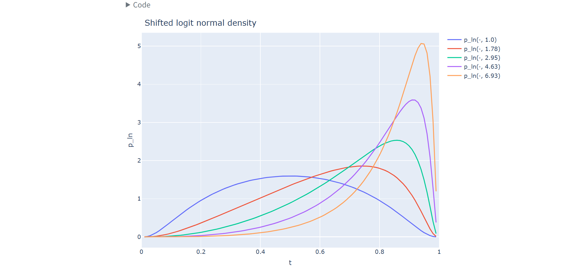
2. Shifted Logit Normal
Define a Gaussian in logit space: \[ z\sim\mathcal{N}(\mu,\sigma^2), \]
and map to \((0,1)\) via the sigmoid: \[ t=\mathrm{sigmoid}(z)=\frac{1}{1+e^{-z}},\quad z=\mathrm{logit}(t)=\log\frac{t}{1-t}. \]
Jacobian (why the denominator has \(t(1-t)\)): \[ \frac{dt}{dz}=t(1-t)\quad\Rightarrow\quad \left|\frac{dz}{dt}\right|=\frac{1}{t(1-t)}. \]
Thus the logit-normal density is \[ p_{\ln}(t;\mu,\sigma)= \frac{1}{\sigma\sqrt{2\pi}\,t(1-t)} \exp\left( -\frac{(\mathrm{logit}(t)-\mu)^2}{2\sigma^2} \right),\quad t\in(0,1). \]
Applying \(\alpha\)-shift as a \(\mu\)-bias
From the logit interpretation: \[ \mathrm{logit}(t')=\mathrm{logit}(t)+\log\alpha. \]
So if \(z=\mathrm{logit}(t)\sim\mathcal{N}(\mu,\sigma^2)\), then \[ z' = z+\log\alpha \sim \mathcal{N}(\mu+\log\alpha,\sigma^2), \] meaning the timeshift is equivalent to shifting the logit-normal mean: \[ t' \sim p_{\ln}(t;\mu+\log\alpha,\sigma). \]
Practical intuition: - Often a strong default distribution. - \(\mu\) controls whether you emphasize low-noise vs high-noise regimes; \(\alpha\) shift simply adds a constant bias in logit space.
3. Plateau Logit Normal
Goal: bias sampling toward higher-noise timesteps by making the density flat after its mode.
Let \(p_{\ln}(t;\mu,\sigma)\) be logit-normal, and define its mode \(t^*\) (numerically solved in the blog code). Define an unnormalized “plateau” density: \[ \tilde{p}_{\mathrm{pln}}(t)= \begin{cases} p_{\ln}(t;\mu,\sigma), & t \le t^*, \\ p_{\ln}(t^*;\mu,\sigma), & t > t^*. \end{cases} \]
Normalize: \[ p_{\mathrm{pln}}(t;\mu,\sigma)=\frac{\tilde{p}_{\mathrm{pln}}(t)}{\int_0^1 \tilde{p}_{\mathrm{pln}}(x)\,dx}. \]
Practical intuition: - Keeps more probability mass in high-noise regions. - In the blog summary, ln/pln frequently beat shifted uniform in best configs.
4. Quick choice guide (one screen)
- If you want a default: try logit-normal (ln) first.
- If you suspect high-noise coverage is undertrained: try plateau logit-normal (pln).
- If you mainly want interpretability / closed-form density: shifted uniform (ts).
Autoencoders
1. Why representations matter (editing vs modeling)
The blog frames AE design around the tension between: - reconstruction fidelity (LPIPS / SSIM / PSNR), - learnability of the latent space for generative modeling, - and compression/efficiency.
For editing, high-fidelity reconstruction is particularly important, but pushing fidelity (e.g., by weakening the bottleneck) can make the latent distribution harder to learn.
2. Metrics (avoid confusion)
- LPIPS / SSIM / PSNR: reconstruction fidelity metrics (input vs reconstructed image).
- rFID: reconstruction FID (reconstruction distribution vs original distribution).
- gFID: generation FID (generated distribution vs real distribution), often used as a proxy for how learnable the latent representation is for the generative backbone.
3. Fair comparison setup (tokenization)
To compare AEs at the same transformer sequence length: - SD / FLUX.1 / FLUX.2 AEs use \(2\times2\) patching on latents, - RAE uses no patching,
so all variants use a consistent sequence length of 256 tokens.
Channels per token in this setup: \[ \text{SD}=16,\quad \text{FLUX.1}=64,\quad \text{FLUX.2}=128,\quad \text{RAE}=768. \]
4. Reconstruction performance (Table 1)
Metrics on ImageNet validation set:
| Model | LPIPS \(\downarrow\) | SSIM \(\uparrow\) | PSNR \(\uparrow\) | rFID \(\downarrow\) |
|---|---|---|---|---|
| RAE | 1.6737 ± 0.0057 | 0.4962 ± 0.0026 | 18.8272 ± 0.0429 | 0.6107 (0.57) |
| SD | 0.9519 ± 0.0054 | 0.6976 ± 0.0121 | 25.0520 ± 0.0673 | 0.6451 (0.62) |
| FLUX.1 | 0.3380 ± 0.0026 | 0.8893 ± 0.0058 | 31.1312 ± 0.0745 | 0.1761 |
| FLUX.2 | 0.2668 ± 0.0017 | 0.9038 ± 0.0049 | 31.4632 ± 0.0633 | 0.1124 |
Quick read: - FLUX.1 and FLUX.2 improve reconstruction strongly over SD. - RAE can have decent rFID-like behavior, but is much worse on reference-based reconstruction fidelity.
5. Why FLUX.1 VAE (Kontext) was “widened”, and the downside
For FLUX.1 Kontext-style editing, FLUX.1 VAE needed higher-fidelity reconstructions. The blog states it was trained with: - 4× larger latent dimensionality, - reduced regularization weight,
which reduces perceptual distortion and helps editing, but also reduces learnability of the latent space.
6. What FLUX.2 VAE changes
FLUX.2 VAE is trained to satisfy editing-level reconstruction fidelity while improving learnability. Key points emphasized in the blog: - reduce compression with an 8× larger dimensionality compared to SD-VAE, - integrate semantic regularization insights (including REPA-related ideas), - resulting in better reconstruction metrics than FLUX.1 VAE while improving learnability.
7. REPA (representation alignment) as a representation knob
REPA is treated as a representation-learning objective that aligns features with a strong vision foundation model. The blog positions REPA-style alignment as a way to regularize representations toward improved learnability, and integrates these insights into FLUX.2 VAE.
Practical guidance from the blog’s parameter study (very condensed)
At 300k steps, the blog compares the impact of different knobs:
- Training distribution (ts vs ln vs pln): ln/pln consistently beat shifted uniform; ln is slightly better for FLUX.2, pln slightly better for RAE.
- Training shift (the \(\alpha\) used during training): highly sensitive; needs to match latent space and training setup.
- Sampling shift: sometimes smaller impact, but still non-trivial for FLUX.2 / RAE.
Scaling up: FLUX.2 model family
FLUX.2 scales on top of the improved representation: - latent flow matching backbone, - unified image generation + editing in one model family, - couples a Mistral-3 24B vision-language model with a rectified-flow transformer, - uses modern activation functions (SwiGLU) and a compute-efficient global modulation mechanism, - operates in the FLUX.2 VAE latent space.
Evaluation headline (Figure 3 in the blog): - text-to-image: 66.6% - multi-reference: 63.6% - single-reference: 59.8%
Background: FFN activations (why “SwiGLU” shows up in FLUX.2)
This section is background to make the line “uses SwiGLU” concrete.
1. Standard Transformer FFN (single-path)
A classic FFN is: \[ \mathrm{FFN}(x)=W_2\,\phi(W_1 x), \] where \(\phi\) is often GELU.
GELU (conceptually): \[ \mathrm{GELU}(x)=x\cdot\Phi(x), \] where \(\Phi\) is the standard normal CDF.
2. SwiGLU as a gated FFN (two-path + elementwise product)
A common Transformer implementation form: \[ \mathrm{SwiGLU}(x)=W_{\mathrm{down}}\Big(\mathrm{SiLU}(W_{\mathrm{gate}}x)\odot(W_{\mathrm{up}}x)\Big). \]
Key point about \(\odot\) (answers the common confusion): - The elementwise product is per token and per channel: - For a token vector \(g,u\in\mathbb{R}^{d_{\mathrm{ff}}}\), \((g\odot u)_i=g_i u_i\). - There is no summation at this multiply step. - The summation (mixing across channels) happens later inside \(W_{\mathrm{down}}\).
Schematic:
x
├─► W_gate ─► SiLU ─┐
│                   ├─► (⊙) ─► W_down ─► out
└─► W_up  ──────────┘
3. SiLU, Swish, and the name “SwiGLU”
Sigmoid: \[ \sigma(x)=\frac{1}{1+e^{-x}}. \]
SiLU (Sigmoid Linear Unit): \[ \mathrm{SiLU}(x)=x\cdot\sigma(x). \]
Swish is the same family with a parameter \(\beta\): \[ \mathrm{Swish}_\beta(x)=x\cdot\sigma(\beta x), \] so SiLU is exactly: \[ \mathrm{SiLU}(x)=\mathrm{Swish}_{\beta=1}(x). \]
Thus “SwiGLU” can be read as: - GLU-style gating (multiplicative interaction), - using Swish/SiLU on the gate branch.
4. Why SwiGLU intermediate width is often “shrunk” (parameter intuition)
Standard FFN uses two projections: \[ \#\text{params}\approx 2 d d_{\mathrm{ff}}. \]
SwiGLU uses three projections: \[ \#\text{params}\approx 3 d d_{\mathrm{ff}}. \]
To keep parameter count comparable, implementations often reduce \(d_{\mathrm{ff}}\) for SwiGLU (commonly around \(\frac{2}{3}\) of the classic “4d” FFN width).
Appendix: SwiGLU MLP snippet (implementation pattern)
1 | class FeedForward(nn.Module): |