FlowAR
FlowAR: Scale-wise Autoregressive Image Generation Meets Flow Matching
Abstract
Recently, in image generation, VAR proposes scale-wise autoregressive modeling, which extends the next token prediction to the next scale prediction, preserving the 2D structure of images. However, VAR encounters two primary challenges: (1) its complex and rigid scale design limits generalization in next scale prediction, and (2) the generator’s dependence on a discrete tokenizer with the same complex scale structure restricts modularity and flexibility in updating the tokenizer.
To address these limitations, we introduce FlowAR, a general next scale prediction method featuring a streamlined scale design, where each subsequent scale is simply double the previous one.
This eliminates the need for VAR’s intricate multi-scale residual tokenizer and enables the use of any off-the-shelf Variational Auto Encoder (VAE).
reference:
VAR:
Tian, K., Jiang, Y., Yuan, Z., Peng, B., and Wang, L. Visual autoregressive modeling: Scalable image generation via next-scale prediction. NeurIPS, 2024
Introduction
Directly applying 1D token-wise autoregressive methods to images presents notable challenges. Images are inherently two-dimensional (2D), with spatial dependencies across height and width. Flattening image tokens disrupts this 2D structure, potentially compromising spatial coherence and causing artifacts in generated images.
Recently, VAR (Tian et al., 2024) addresses these issues by introducing scale-wise autoregressive modeling, which progressively generates images from coarse to fine scales, preserving the spatial hierarchies and dependencies essential for visual coherence.
Despite its effectiveness, VAR (Tian et al., 2024) faces two significant limitations: (1) a complex and rigid scale design, and (2) a dependency between the generator and a tokenizer that shares this intricate scale structure. Specifically, VAR employs a non-uniform scale sequence, \(\{1,2,3,4,5,6,8,10,13,16\}\), where the coarsest scale tokenizes a \(256 \times 256\) image into a single \(1 \times 1\) token and the finest scale into \(16 \times 16\) tokens. This intricate sequence constrains both the tokenizer and generator to operate exclusively at these predefined scales, limiting adaptability to other resolutions or granularities. Consequently, the model struggles to represent or generate features that fall outside this fixed scale sequence. Additionally, the tight coupling between VAR's generator and tokenizer restricts flexibility in independently updating the tokenizer, as both components must adhere to the same scale structure.
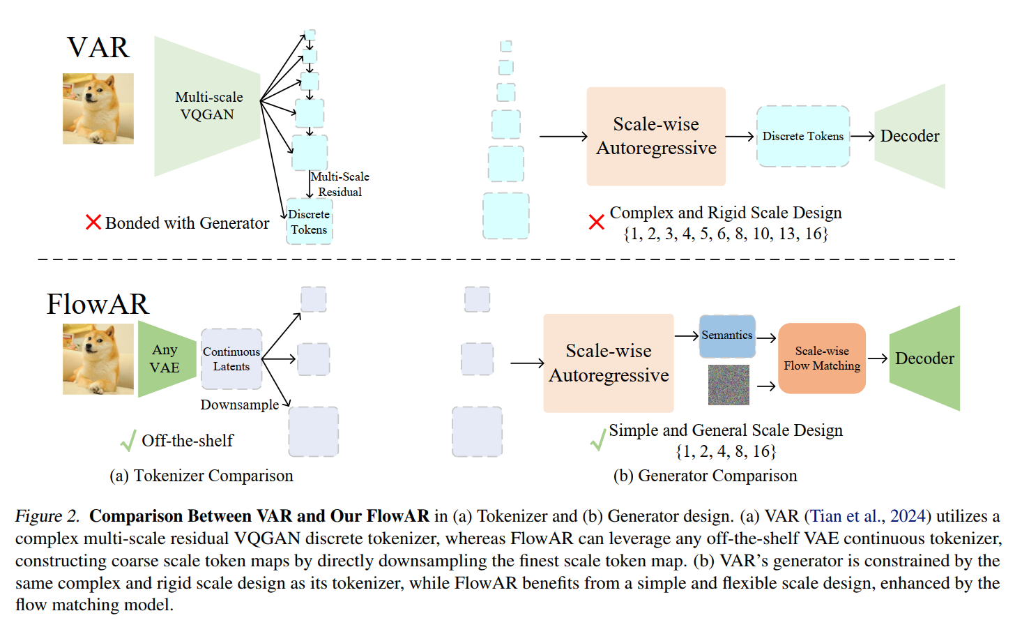
To address these limitations, we introduce FlowAR, a flexible and generalized approach to scale-wise autoregressive modeling for image generation, enhanced with flow matching (Lipman et al., 2022). Unlike VAR (Tian et al., 2024), which relies on a complex multi-scale VQGAN discrete tokenizer (Razavi et al., 2019; Lee et al., 2022), we utilize any off-the-shelf VAE continuous tokenizer (Kingma & Welling, 2014) with a simplified scale design, where each subsequent scale is simply double the previous one (e.g., \(\{1,2,4,8,16\})\), and coarse scale tokens are obtained by directly downsampling the finest scale tokens (i.e., the largest resolution token map). This streamlined design eliminates the need for a specially designed tokenizer and decouples the tokenizer from the generator, allowing greater flexibility to update the tokenizer with any modern VAE (Li et al., 2024; Chen et al., 2024).
To further enhance image quality, we incorporate the flow matching model (Lipman et al., 2022) to learn the probability distribution at each scale. Specifically, given the class token and tokens from previous scales, we use an autoregressive Transformer (Radford et al., 2018) to generate continuous semantics that condition the flow matching model, progressively transforming noise into the target latent representation for the current scale. Conditioning is achieved through the proposed spatially adaptive layer normalization (Spatial-adaLN), which adaptively adjusts layer normalization (Ba et al., 2016) on a position-by-position basis, capturing fine-grained details and improving the model's ability to generate high-fidelity images. This process is repeated across scales, capturing the hierarchical dependencies inherent in natural images.
Method
VAR
Scale-wise Autoregressive Modeling for Image
Generation. Rather than flattening images into token sequences,
VAR (Tian et al., 2024) decomposes the image into a series of token maps
across multiple scales, \(S=\left\{s_1, s_2,
\ldots, s_n\right\}\). Each token map \(s_k\) has dimensions \(h_k \times w_k\) and is obtained by a
specially designed multi-scale VQGAN with residual structure (Razavi et
al., 2019; Lee et al., 2022; Tian et al., 2024; Esser et al., 2021). In
contrast to single flattened tokens \(t_k\) that lose spatial context,
each \(s_k\) maintains the
two-dimensional structure with \(h_k \times
w_k\) tokens. The autoregressive loss function is then
reformulated to predict each scale based on all preceding scales:
\[
\mathcal{L}=-\sum_{k=1}^n \log p\left(s_k \mid s_{<k}, \Theta\right)
\] In this framework, generating the \(k\)-th scale in VAR requires attending to
all previous scales \(s_{<k}\)
(i.e., \(s_1\) to \(\left.s_{k-1}\right)\) and simultaneously
predicting all \(h_k \times w_k\)
tokens in \(s_k\) via categorical
distributions. The chosen scales, \(S=\{1,2,3,4,5,6,8,10,13,16\}\), introduce
significant complexity to the scale design and constrain the model's
generalization capabilities. This is due to the tight coupling between
the generator and tokenizer with the scale design, reducing flexibility
in updating the tokenizer or supporting alternative scale
configurations. Furthermore, VAR's discrete tokenizer relies on a
complex multi-scale residual structure, complicating the training
process, with essential training code and details remaining publicly
unavailable at the time of our submission.
FlowAR
Our method incorporates two primary improvements over existing next scale prediction:
- replacing the multi-scale VQGAN discrete tokenizer with any off-the-shelf VAE continuous tokenizer
- modeling the per-scale prediction (i.e., predicting all \(hk \times wk\) tokens in \(k\)-th scale \(sk\)) using flow matching to learn the probability distribution.
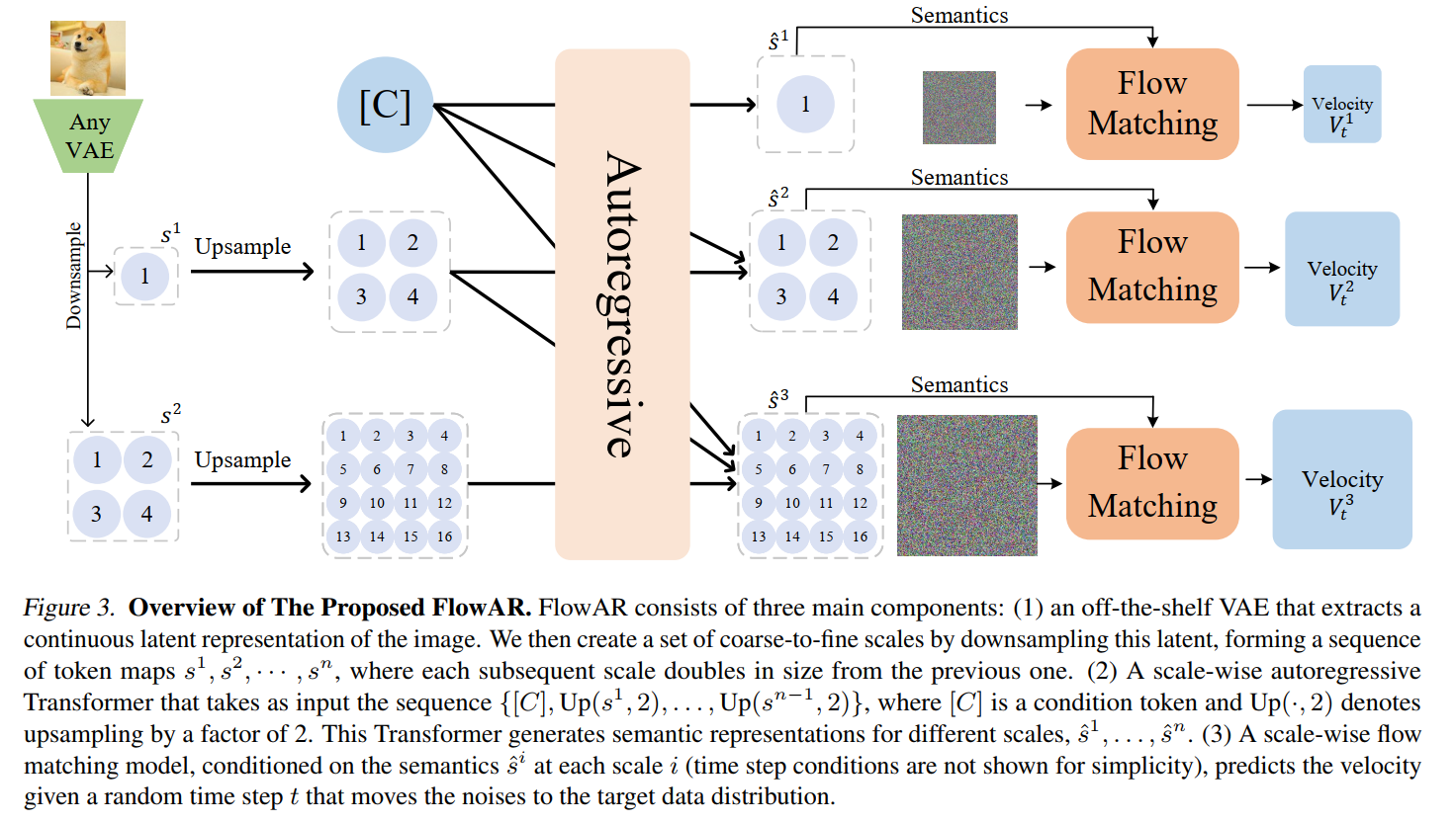
Simple Scale Sequence with Any VAE Tokenizer: we extract its continuous latent representation using an off-the-shelf VAE, we then construct a set of coarse-to-fine scales by downsampling the latent \(F\) as a factor of 2 sequentially. We utilize the Transformer to generate conditioning information for each scale, while a scale-wise flow matching model captures the scale’s probability distribution based on this information.
Generating Conditioning Information via Scale-wise Autoregressive Transformer: To produce the conditioning information for each subsequent scale, we utilize conditions obtained from all previous scales \[ \hat{s}^i=T\left(\left[C, \mathrm{Up}\left(s^1, 2\right), \ldots, \mathrm{Up}\left(s^{i-1}, 2\right)\right]\right), \forall i=1, \cdots, n, \] where \(T(\cdot)\) represents the autoregressive Transformer model, \(C\) is the class condition, and \(\mathrm{Up}(s, r)\) denotes the up-sampling of latent \(s\) by a factor of \(r\). For the initial scale \((i=1)\), only the class condition \(C\) is used as input. We set \(r=2\), following our simple scale design, where each scale is double the size of the previous one. We refer to the resulting output \(\hat{s}^i\) as the semantics for the \(i\)-th scale, which is then used to condition a flow matching module to learn the per-scale probability distribution.
Scale-wise Flow Matching Model Conditioned by Autoregressive Transformer Output. For each \(i\)-th scale, FlowAR extends flow matching to generate the scale latent \(s^i\), conditioned on the autoregressive Transformer's output \(\hat{s}^i\). ... Unlike prior approaches (Atito et al., 2021; Esser et al., 2024) that condition velocity prediction on class or textual information, we condition on the scale-wise semantics \(\hat{s}^i\) from the autoregressive Transformer’s output. Notably, in prior methods (Atito et al., 2021; Esser et al., 2024), the conditions and image latents often have different lengths, whereas FlowAR shares the same length (i.e., \(s^i\) and \(\hat{s}^i\) have the same shape, \(\forall i=1, \cdots, n\) ). The training objective for scale-wise flow matching is: \[ \mathcal{L}=\sum_{i=1}^n\left\|\mathrm{FM}\left(F_t^i, \hat{s}^i, t ; \theta\right)-V_t^i\right\|^2, \] where FM denotes the flow matching model parameterized by \(\theta\). This approach allows the model to capture scale-wise information bi-directionally, enhancing flexibility and efficiency in image generation within our framework.
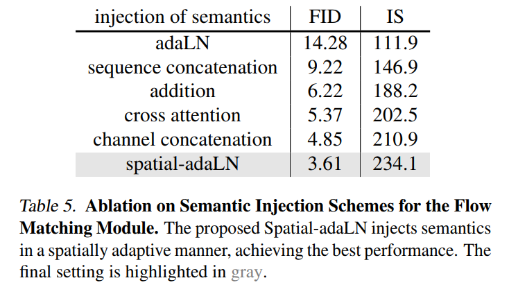
Scale-wise Injection of Semantics via Spatial-adaLN. A key design choice is determining how best to inject the semantic information \(\hat{s}^i\), generated by the autoregressive Transformer, into the flow matching module. A straightforward approach would be to concatenate the semantics \(\hat{s}^i\) with the flattened input \(F_t^i\), similar to in-context conditioning (Bao et al., 2023) where the class condition is concatenated with the input sequence. However, this approach has two main drawbacks: (1) it increases the sequence length input to the flow matching model, raising computational costs, and (2) it provides indirect semantic injection, potentially weakening the effectiveness of semantic guidance. To address these issues, we propose using spatially adaptive layer-norm for position-by-position semantic injection, resulting in the proposed Spatial-adaLN. Specifically, given the semantics \(\hat{s}^i\) from the scale-wise autoregressive Transformer and the intermediate feature \(F_t^{i^{\prime}}\) in the flow matching model, we inject the semantics to the scale \(\gamma\), shift \(\beta\), and gate \(\alpha\) parameters of the adaptive normalization, following the standard adaptive normalization procedure (Ba et al., 2016; Zhang & Sennrich, 2019; Peebles & Xie, 2023): \[ \begin{aligned} \alpha_1, \alpha_2, \beta_1, \beta_2, \gamma_1, \gamma_2 & =\operatorname{MLP}\left(\hat{s}^i+t\right) \\ \hat{F}_t^{i^{\prime}} & =\operatorname{Attn}\left(\gamma_1 \odot \operatorname{LN}\left(F_t^{i^{\prime}}\right)+\beta_1\right) \odot \alpha_1 \\ F_t^{i^{\prime \prime}} & =\operatorname{MLP}\left(\gamma_2 \odot \operatorname{LN}\left(\hat{F}_t^{i^{\prime}}\right)+\beta_2\right) \odot \alpha_2 \end{aligned} \]
where Attn denotes the attention mechanism, and LN denotes the layer norm, \(F_t^{i^{\prime \prime}}\) is the block's output, and \(\odot\) is the spatial-wise product. Unlike traditional adaptive normalization, where the scale, shift, and gate parameters lack spatial information, our spatial adaptive normalization provides positional control, enabling dependency on semantics from the
Inference Pipeline. At the beginning of inference, the autoregressive Transformer generates the initial semantics \(\hat{s}^1\) using only the class condition \(C\). This semantics \(\hat{s}^1\) conditions the flow matching module, which gradually transforms a noise sample into the target distribution for \(s^1\). The resulting token map is upsampled by a factor of 2 , combined with the class condition, and fed back into the autoregressive Transformer to generate the semantics \(\hat{s}^2\), which conditions the flow matching module for the next scale. This process is iterated \(n\) scales until the final token map \(s^n\) is estimated and subsequently decoded by the VAE decoder to produce the generated image. Notably, we use the KV cache (Pope et al., 2023) in the autoregressive Transformer to efficiently generate each semantics \(\hat{s}^i\).
Experimental results
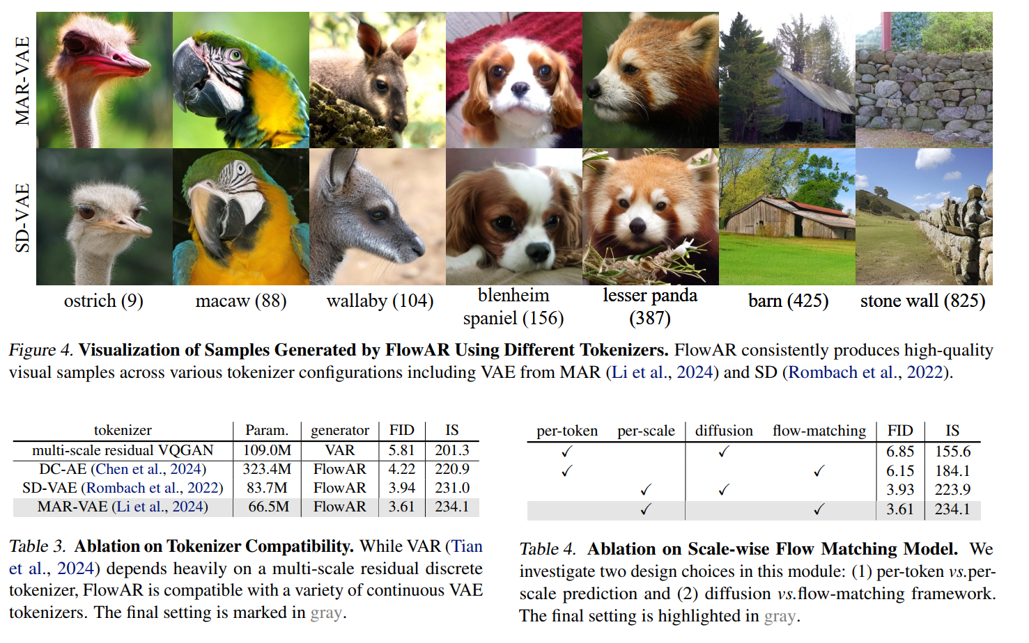
Ablation Studies